单细胞数据初步处理 | drop-seq | QC | 质控 | 正则化 normalization

比对

The raw Drop-seq data was processed with the standard pipeline (Drop-seq tools version 1.12 from McCarroll laboratory). Reads were aligned to the ENSEMBL release 84Mus musculusgenome.

10x Genomics data was processed using the same pipeline as for Drop-seq data, adjusting the barcode locations accordingly

我还没有深入接触10x和drop-seq的数据，目前的10x数据都是用官网cellranger跑出来的。

质控

We selected cells for downstream processing in each Drop-seq run, using the quality control metrics output by the Drop-seq tools package9, as well as metrics derived from the UMI matrix.

1) We first removed cells with a low number (<700) of unique detected genes. From the remaining cells, we filtered additional outliers.

2) We removed cells for which the overall alignment rate was less than the mean minus three standard deviations.

3) We removed cells for which the total number of reads (after log10 transformation) was not within three standard deviations of the mean.

4) We removed cells for which the total number of unique molecules (UMIs, after log10 transformation) was not within three standard deviations of the mean.

5) We removed cells for which the transcriptomic alignment rate (defined by PCT_USABLE_BASES) was not within three standard deviations of the mean.

6) We removed cells that showed an unusually high or low number of UMIs given their number of reads by fitting a loess curve (span= 0.5, degree= 2) to the number of UMIs with number of reads as predictor (both after log10 transformation). Cells with a residual more than three standard deviations away from the mean were removed.

7) With the same criteria, we removed cells that showed an unusually high or low number of genes given their number of UMIs. Of these filter steps, step 1 removed the majority of cells.

Steps 2 to 7 removed only a small number of additional cells from each eminence (2% to 4%), and these cells did not exhibit unique or biologically informative patterns of gene expression.

1. 过滤掉基因数量太少的细胞；

2. 过滤基因组比对太差的细胞；

3. 过滤掉总reads数太少的细胞；

4. 过滤掉UMI太少的细胞；

5. 过滤掉转录本比对太少的细胞；

6. 根据统计分析，过滤reads过多或过少的细胞；

7. 根据统计分析，过滤UMI过低或过高的细胞；

注：连过滤都有点统计的门槛，其实也简单，应该是默认为正态分布，去掉了左右极端值。

还有一个就是简单的拟合回归，LOESS Curve Fitting (Local Polynomial Regression)

How to fit a smooth curve to my data in R?

正则化

The raw data per Drop-seq run is a UMI count matrix with genes as rows and cells as columns. The values represent the number of UMIs that were detected. The aim of normalization is to make these numbers comparable between cells by removing the effect of sequencing depth and biological sources of heterogeneity that may confound the signal of interest, in our case cell cycle stage.

目前有很多正则化的方法，但是作者还是自己开发了一个。

正则化就是去掉一些影响因素，使得我们的数据之间可以相互比较。这里就提到了两个最主要的因素：测序深度和细胞周期。

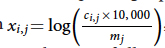
A common approach to correct for sequencing depth is to create a new normalized expression matrix x with (see Fig), in which ci,j is the molecule count of gene i in cell j and mj is the sum of all molecule counts for cell j. This approach assumes that ci,j increases linearly with mj, which is true only when the set of genes detected in each cell is roughly the same.

可以看到常规的正则化方法是不适合的，

However, for Drop-seq, in which the number of UMIs is low per cell compared to the number of genes present, the set of genes detected per cell can be quite different. Hence, we normalize the expression of each gene separately by modelling the UMI counts as coming from a generalized linear model with negative binomial distribution, the mean of which can be dependent on technical factors related to sequencing depth. Specifically, for every gene we model the expected value of UMI counts as a function of the total number of reads assigned to that cell, and the number of UMIs per detected gene (sum of UMI divided by number of unique detected genes).

这个就有些门槛了，用了广义线性回归模型来做正则化。

To solve the regression problem, we use a generalized linear model (glm function of base R package) with a regularized overdispersion parameter theta. Regularizing theta helps us to avoid overfitting which could occur for genes whose variability is mostly driven by biological processes rather than sampling noise and dropout events. To learn a regularized theta for every gene, we perform the following procedure.

1) For every gene, obtain an empirical theta using the maximum likelihood model (theta.ml function of the MASS R package) and the estimated mean vector that is obtained by a generalized linear model with Poisson error distribution.

2) Fit a line (loess, span = 0.33, degree = 2) through the variance–mean UMI count relationship (both log10 transformed) and predict regularized theta using the fit. The relationship between variance and theta and mean is given by variance= mean + (mean2/theta).
Normalized expression is then defined as the Pearson residual of the regression model, which can be interpreted as the number of standard deviations by which an observed UMI count was higher or lower than its expected value. Unless stated otherwise, we clip expression to the range [-30, 30] to prevent outliers from dominating downstream analyses.

好的是，代码人家都给出来了，你去跑跑，就能猜出大致的意思。

# for normalization
# regularized overdispersion parameter theta. Regularizing theta helps us to avoid overfitting which could occur for genes whose variability is mostly driven by biological processes rather than sampling noise and dropout events.
# divide all genes into 64 bins
theta.reg <- function(cm, regressors, min.theta=0.01, bins=64) {
  b.id <- (1:nrow(cm)) %% max(1, bins, na.rm=TRUE) + 1
  cat(sprintf('get regularized theta estimate for %d genes and %d cells\n', nrow(cm), ncol(cm)))
  cat(sprintf('processing %d bins with ca %d genes in each\n', bins, round(nrow(cm)/bins, 0)))
  theta.estimate <- rep(NA, nrow(cm))
  # For every gene, obtain an empirical theta using the maximum likelihood model (theta.ml function of the MASS R package)
  for (bin in sort(unique(b.id))) {
    sel.g <- which(b.id == bin)
    bin.theta.estimate <- unlist(mclapply(sel.g, function(i) {
      # estimated mean vector that is obtained by a generalized linear model with Poisson error distribution
      as.numeric(theta.ml(cm[i, ], glm(cm[i, ] ~ ., data = regressors, family=poisson)$fitted))
    }), use.names = FALSE)
    theta.estimate[sel.g] <- bin.theta.estimate
    cat(sprintf('%d ', bin))
  }
  cat('done\n')
  raw.mean <- apply(cm, 1, mean)
  log.raw.mean <- log10(raw.mean)
  var.estimate <- raw.mean + raw.mean^2/theta.estimate

  # Fit a line (loess, span = 0.33, degree = 2) through the variance–mean UMI count relationship (both log10 transformed)
  fit <- loess(log10(var.estimate) ~ log.raw.mean, span=0.33)
  # predict regularized theta using the fit. The relationship between variance and theta and mean is given by variance= mean + (mean2/theta)
  theta.fit <- raw.mean^2 / (10^fit$fitted - raw.mean)

  to.fix <- theta.fit <= min.theta | is.infinite(theta.fit)
  if (any(to.fix)) {
    cat('Fitted theta below', min.theta, 'for', sum(to.fix), 'genes, setting them to', min.theta, '\n')
    theta.fit[to.fix] <- min.theta
  }
  names(theta.fit) <- rownames(cm)
  return(theta.fit)
}

nb.residuals.glm <- function(y, regression.mat, fitted.theta, gene) {
  fit <- 0
  try(fit <- glm(y ~ ., data = regression.mat, family=negative.binomial(theta=fitted.theta)), silent=TRUE)
  if (class(fit)[1] == 'numeric') {
    message(sprintf('glm and family=negative.binomial(theta=%f) failed for gene %s; falling back to scale(log10(y+1))',
                    fitted.theta, gene))
    return(scale(log10(y+1))[, 1])
  }
  return(residuals(fit, type='pearson'))
}

## Main function
norm.nb.reg <- function(cm, regressors, min.theta=0.01, bins=64, theta.fit=NA, pr.th=NA, save.theta.fit=c()) {
  cat('Normalizing data using regularized NB regression\n')
  cat('explanatory variables:', colnames(regressors), '\n')
  if (any(is.na(theta.fit))) {
    theta.fit <- theta.reg(cm, regressors, min.theta, bins)
    if (is.character(save.theta.fit)) {
      save(theta.fit, file=save.theta.fit)
    }
  }

  b.id <- (1:nrow(cm)) %% max(1, bins, na.rm=TRUE) + 1
  cat('Running NB regression\n')
  res <- matrix(NA, nrow(cm), ncol(cm), dimnames=dimnames(cm))
  for (bin in sort(unique(b.id))) {
    sel.g <- rownames(cm)[b.id == bin]
    expr.lst <- mclapply(sel.g, function(gene) nb.residuals.glm(cm[gene, ], regressors, theta.fit[gene], gene), mc.preschedule = TRUE)
    # Normalized expression is then defined as the Pearson residual of the regression model, which can be interpreted as the number of standard deviations by which an observed UMI count was higher or lower than its expected value.
    res[sel.g, ] <- do.call(rbind, expr.lst)
    cat(sprintf('%d ', bin))
  }
  cat('done\n')
  # clip expression to the range [-30, 30] to prevent outliers from dominating downstream analyses
  if (!any(is.na(pr.th))) {
    res[res > pr.th] <- pr.th
    res[res < -pr.th] <- -pr.th
  }
  attr(res, 'theta.fit') <- theta.fit
  return(res)
}