机器学习（ML）一之 Linear Regression

一、线性回归

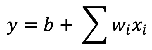
1、模型

2、损失函数

3、优化函数-梯度下降

#!/usr/bin/env python
# coding: utf-8
import torch
import time

# init variable a, b as 1000 dimension vector
n = 1000
a = torch.ones(n)
b = torch.ones(n)

# define a timer class to record time
class Timer(object):
    """Record multiple running times."""
    def __init__(self):
        self.times = []
        self.start()

    def start(self):
        # start the timer
        self.start_time = time.time()

    def stop(self):
        # stop the timer and record time into a list
        self.times.append(time.time() - self.start_time)
        return self.times[-1]

    def avg(self):
        # calculate the average and return
        return sum(self.times)/len(self.times)

    def sum(self):
        # return the sum of recorded time
        return sum(self.times)

timer = Timer()
c = torch.zeros(n)
for i in range(n):
    c[i] = a[i] + b[i]
'%.5f sec' % timer.stop()

timer.start()
d = a + b
'%.5f sec' % timer.stop()

# import packages and modules
get_ipython().run_line_magic('matplotlib', 'inline')
import torch
from IPython import display
from matplotlib import pyplot as plt
import numpy as np
import random

print(torch.__version__)

# ### 线性回归模型从零开始的实现

# set input feature number
num_inputs = 2
# set example number
num_examples = 1000

# set true weight and bias in order to generate corresponded label
true_w = [2, -3.4]
true_b = 4.2

features = torch.randn(num_examples, num_inputs,
                      dtype=torch.float32)
labels = true_w[0] * features[:, 0] + true_w[1] * features[:, 1] + true_b
labels += torch.tensor(np.random.normal(0, 0.01, size=labels.size()),
                       dtype=torch.float32)

# ### 使用图像来展示生成的数据

plt.scatter(features[:, 1].numpy(), labels.numpy(), 1);

# ### 读取数据集

def data_iter(batch_size, features, labels):
    num_examples = len(features)
    indices = list(range(num_examples))
    random.shuffle(indices)  # random read 10 samples
    for i in range(0, num_examples, batch_size):
        j = torch.LongTensor(indices[i: min(i + batch_size, num_examples)]) # the last time may be not enough for a whole batch
        yield  features.index_select(0, j), labels.index_select(0, j)

batch_size = 10

for X, y in data_iter(batch_size, features, labels):
    print(X, '\n', y)
    break

# ### 模型初始化

w = torch.tensor(np.random.normal(0, 0.01, (num_inputs, 1)), dtype=torch.float32)
b = torch.zeros(1, dtype=torch.float32)

w.requires_grad_(requires_grad=True)
b.requires_grad_(requires_grad=True)

# ### 定义模型
# 定义用来训练参数的训练模型：
# $$ \mathrm{price} = w_{\mathrm{area}} \cdot \mathrm{area} + w_{\mathrm{age}} \cdot \mathrm{age} + b $$

# In[19]:

def linreg(X, w, b):
    return torch.mm(X, w) + b

# ### 定义损失函数
# 我们使用的是均方误差损失函数：
# $$l^{(i)}(\mathbf{w}, b) = \frac{1}{2} \left(\hat{y}^{(i)} - y^{(i)}\right)^2,$$

# In[16]:

def squared_loss(y_hat, y):
    return (y_hat - y.view(y_hat.size())) ** 2 / 2

# ### 定义优化函数
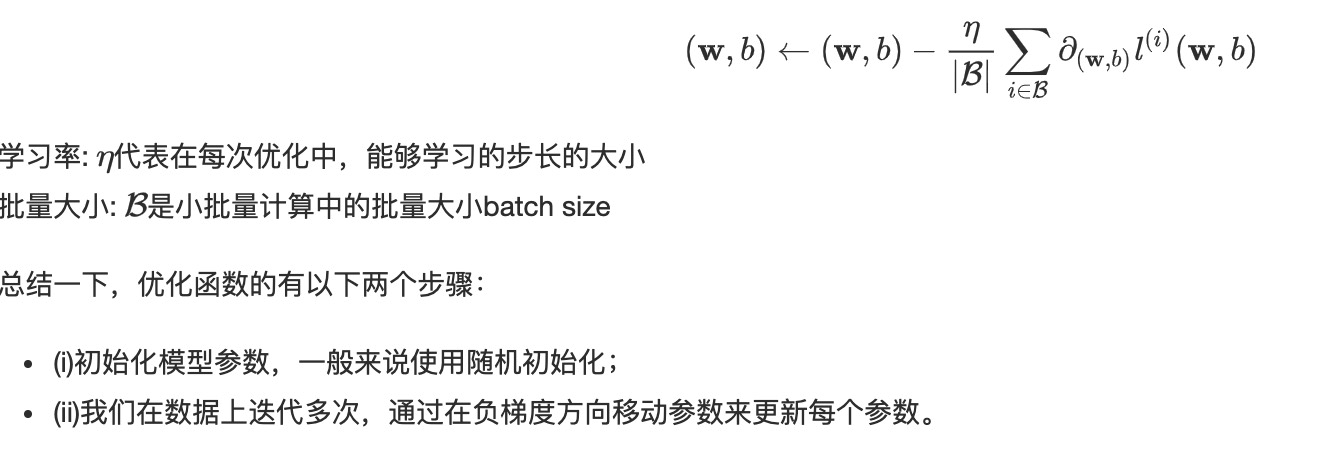
# 在这里优化函数使用的是小批量随机梯度下降：
# $$(\mathbf{w},b) \leftarrow (\mathbf{w},b) - \frac{\eta}{|\mathcal{B}|} \sum_{i \in \mathcal{B}} \partial_{(\mathbf{w},b)} l^{(i)}(\mathbf{w},b)$$

# In[17]:

def sgd(params, lr, batch_size):
    for param in params:
        param.data -= lr * param.grad / batch_size # ues .data to operate param without gradient track

# ### 训练
# 当数据集、模型、损失函数和优化函数定义完了之后就可来准备进行模型的训练了。

# In[20]:

# super parameters init
lr = 0.03
num_epochs = 5

net = linreg
loss = squared_loss

# training
for epoch in range(num_epochs):  # training repeats num_epochs times
    # in each epoch, all the samples in dataset will be used once

    # X is the feature and y is the label of a batch sample
    for X, y in data_iter(batch_size, features, labels):
        l = loss(net(X, w, b), y).sum()
        # calculate the gradient of batch sample loss
        l.backward()
        # using small batch random gradient descent to iter model parameters
        sgd([w, b], lr, batch_size)
        # reset parameter gradient
        w.grad.data.zero_()
        b.grad.data.zero_()
    train_l = loss(net(features, w, b), labels)
    print('epoch %d, loss %f' % (epoch + 1, train_l.mean().item()))

# In[21]:

w, true_w, b, true_b

# ### 线性回归模型使用pytorch的简洁实现

# In[22]:

import torch
from torch import nn
import numpy as np
torch.manual_seed(1)

print(torch.__version__)
torch.set_default_tensor_type('torch.FloatTensor')

# ### 生成数据集
# 在这里生成数据集跟从零开始的实现中是完全一样的。

# In[23]:

num_inputs = 2
num_examples = 1000

true_w = [2, -3.4]
true_b = 4.2

features = torch.tensor(np.random.normal(0, 1, (num_examples, num_inputs)), dtype=torch.float)
labels = true_w[0] * features[:, 0] + true_w[1] * features[:, 1] + true_b
labels += torch.tensor(np.random.normal(0, 0.01, size=labels.size()), dtype=torch.float)

# ### 读取数据集

# In[24]:

import torch.utils.data as Data

batch_size = 10

# combine featues and labels of dataset
dataset = Data.TensorDataset(features, labels)

# put dataset into DataLoader
data_iter = Data.DataLoader(
    dataset=dataset,            # torch TensorDataset format
    batch_size=batch_size,      # mini batch size
    shuffle=True,               # whether shuffle the data or not
    num_workers=2,              # read data in multithreading
)

# In[27]:

for X, y in data_iter:
    print(X, '\n', y)
    break

# ### 定义模型

# In[28]:

class LinearNet(nn.Module):
    def __init__(self, n_feature):
        super(LinearNet, self).__init__()      # call father function to init
        self.linear = nn.Linear(n_feature, 1)  # function prototype: `torch.nn.Linear(in_features, out_features, bias=True)`

    def forward(self, x):
        y = self.linear(x)
        return y

net = LinearNet(num_inputs)
print(net)

# In[29]:

# ways to init a multilayer network
# method one
net = nn.Sequential(
    nn.Linear(num_inputs, 1)
    # other layers can be added here
    )

# method two
net = nn.Sequential()
net.add_module('linear', nn.Linear(num_inputs, 1))
# net.add_module ......

# method three
from collections import OrderedDict
net = nn.Sequential(OrderedDict([
          ('linear', nn.Linear(num_inputs, 1))
          # ......
        ]))

print(net)
print(net[0])

# ### 初始化模型参数

# In[30]:

from torch.nn import init

init.normal_(net[0].weight, mean=0.0, std=0.01)
init.constant_(net[0].bias, val=0.0)  # or you can use `net[0].bias.data.fill_(0)` to modify it directly

# In[31]:

for param in net.parameters():
    print(param)

# ### 定义损失函数

# In[32]:

loss = nn.MSELoss()    # nn built-in squared loss function
                       # function prototype: `torch.nn.MSELoss(size_average=None, reduce=None, reduction='mean')`

# ### 定义优化函数

# In[33]:

import torch.optim as optim

optimizer = optim.SGD(net.parameters(), lr=0.03)   # built-in random gradient descent function
print(optimizer)  # function prototype: `torch.optim.SGD(params, lr=, momentum=0, dampening=0, weight_decay=0, nesterov=False)`

# In[34]:

##trainning
num_epochs = 3
for epoch in range(1, num_epochs + 1):
    for X, y in data_iter:
        output = net(X)
        l = loss(output, y.view(-1, 1))
        optimizer.zero_grad() # reset gradient, equal to net.zero_grad()
        l.backward()
        optimizer.step()
    print('epoch %d, loss: %f' % (epoch, l.item()))

# In[35]:

# result comparision
dense = net[0]
print(true_w, dense.weight.data)
print(true_b, dense.bias.data)

# In[ ]: