吴裕雄 python 机器学习——核化PCAKernelPCA模型

# -*- coding: utf-8 -*-

import numpy as np
import matplotlib.pyplot as plt

from sklearn import datasets,decomposition

def load_data():
    '''
    加载用于降维的数据
    '''
    # 使用 scikit-learn 自带的 iris 数据集
    iris=datasets.load_iris()
    return iris.data,iris.target

#核化PCAKernelPCA模型
def test_KPCA(*data):
    X,y=data
    kernels=['linear','poly','rbf','sigmoid']
    # 依次测试四种核函数
    for kernel in kernels:
        kpca=decomposition.KernelPCA(n_components=None,kernel=kernel)
        kpca.fit(X)
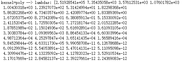
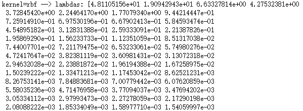
        print('kernel=%s --> lambdas: %s'% (kernel,kpca.lambdas_))

# 产生用于降维的数据集
X,y=load_data()
# 调用 test_KPCA
test_KPCA(X,y) 

...................

....................

def plot_KPCA(*data):
    '''
    绘制经过 KernelPCA 降维到二维之后的样本点
    '''
    X,y=data
    kernels=['linear','poly','rbf','sigmoid']
    fig=plt.figure()
    # 颜色集合，不同标记的样本染不同的颜色
    colors=((1,0,0),(0,1,0),(0,0,1),(0.5,0.5,0),(0,0.5,0.5),(0.5,0,0.5),(0.4,0.6,0),(0.6,0.4,0),(0,0.6,0.4),(0.5,0.3,0.2))

    for i,kernel in enumerate(kernels):
        kpca=decomposition.KernelPCA(n_components=2,kernel=kernel)
        kpca.fit(X)
        # 原始数据集转换到二维
        X_r=kpca.transform(X)
        ## 两行两列，每个单元显示一种核函数的 KernelPCA 的效果图
        ax=fig.add_subplot(2,2,i+1)
        for label ,color in zip( np.unique(y),colors):
            position=y==label
            ax.scatter(X_r[position,0],X_r[position,1],label="target= %d"%label,
            color=color)
        ax.set_xlabel("X[0]")
        ax.set_ylabel("X[1]")
        ax.legend(loc="best")
        ax.set_title("kernel=%s"%kernel)
    plt.suptitle("KPCA")
    plt.show()

# 调用 plot_KPCA
plot_KPCA(X,y)   

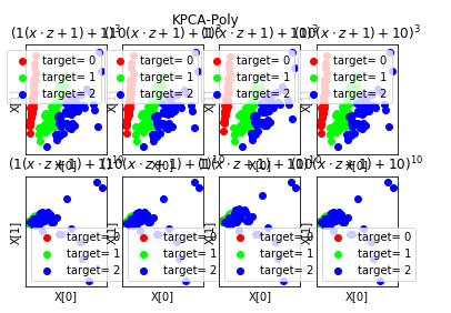
def plot_KPCA_poly(*data):
    '''
    绘制经过 使用 poly 核的KernelPCA 降维到二维之后的样本点
    '''
    X,y=data
    fig=plt.figure()
    # 颜色集合，不同标记的样本染不同的颜色
    colors=((1,0,0),(0,1,0),(0,0,1),(0.5,0.5,0),(0,0.5,0.5),(0.5,0,0.5),(0.4,0.6,0),(0.6,0.4,0),(0,0.6,0.4),(0.5,0.3,0.2))
    # poly 核的参数组成的列表。
    # 每个元素是个元组，代表一组参数（依次为：p 值， gamma 值， r 值）
    # p 取值为：3，10
    # gamma 取值为 ：1，10
    # r 取值为：1，10
    # 排列组合一共 8 种组合
    Params=[(3,1,1),(3,10,1),(3,1,10),(3,10,10),(10,1,1),(10,10,1),(10,1,10),(10,10,10)]
    for i,(p,gamma,r) in enumerate(Params):
        # poly 核，目标为2维
        kpca=decomposition.KernelPCA(n_components=2,kernel='poly',gamma=gamma,degree=p,coef0=r)
        kpca.fit(X)
        # 原始数据集转换到二维
        X_r=kpca.transform(X)
        ## 两行四列，每个单元显示核函数为 poly 的 KernelPCA 一组参数的效果图
        ax=fig.add_subplot(2,4,i+1)
        for label ,color in zip( np.unique(y),colors):
            position=y==label
            ax.scatter(X_r[position,0],X_r[position,1],label="target= %d"%label,
            color=color)
        ax.set_xlabel("X[0]")
        # 隐藏 x 轴刻度
        ax.set_xticks([])
        # 隐藏 y 轴刻度
        ax.set_yticks([])
        ax.set_ylabel("X[1]")
        ax.legend(loc="best")
        ax.set_title(r"$ (%s (x \cdot z+1)+%s)^{%s}$"%(gamma,r,p))
    plt.suptitle("KPCA-Poly")
    plt.show()

# 调用 plot_KPCA_poly
plot_KPCA_poly(X,y)   

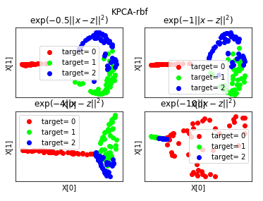
def plot_KPCA_rbf(*data):
    '''
    绘制经过 使用 rbf 核的KernelPCA 降维到二维之后的样本点
    '''
    X,y=data
    fig=plt.figure()
    # 颜色集合，不同标记的样本染不同的颜色
    colors=((1,0,0),(0,1,0),(0,0,1),(0.5,0.5,0),(0,0.5,0.5),(0.5,0,0.5),(0.4,0.6,0),(0.6,0.4,0),(0,0.6,0.4),(0.5,0.3,0.2))
    # rbf 核的参数组成的列表。每个参数就是 gamma值
    Gammas=[0.5,1,4,10]
    for i,gamma in enumerate(Gammas):
        kpca=decomposition.KernelPCA(n_components=2,kernel='rbf',gamma=gamma)
        kpca.fit(X)
        # 原始数据集转换到二维
        X_r=kpca.transform(X)
        ## 两行两列，每个单元显示核函数为 rbf 的 KernelPCA 一组参数的效果图
        ax=fig.add_subplot(2,2,i+1)
        for label ,color in zip( np.unique(y),colors):
            position=y==label
            ax.scatter(X_r[position,0],X_r[position,1],label="target= %d"%label,
            color=color)
        ax.set_xlabel("X[0]")
        # 隐藏 x 轴刻度
        ax.set_xticks([])
        # 隐藏 y 轴刻度
        ax.set_yticks([])
        ax.set_ylabel("X[1]")
        ax.legend(loc="best")
        ax.set_title(r"$\exp(-%s||x-z||^2)$"%gamma)
    plt.suptitle("KPCA-rbf")
    plt.show()

# 调用 plot_KPCA_rbf
plot_KPCA_rbf(X,y)   

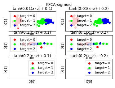
def plot_KPCA_sigmoid(*data):
    '''
    绘制经过 使用 sigmoid 核的KernelPCA 降维到二维之后的样本点
    '''
    X,y=data
    fig=plt.figure()
    # 颜色集合，不同标记的样本染不同的颜色
    colors=((1,0,0),(0,1,0),(0,0,1),(0.5,0.5,0),(0,0.5,0.5),(0.5,0,0.5),(0.4,0.6,0),(0.6,0.4,0),(0,0.6,0.4),(0.5,0.3,0.2))
    # sigmoid 核的参数组成的列表。
    Params=[(0.01,0.1),(0.01,0.2),(0.1,0.1),(0.1,0.2),(0.2,0.1),(0.2,0.2)]
        # 每个元素就是一种参数组合（依次为 gamma,coef0）
        # gamma 取值为： 0.01，0.1，0.2
        # coef0 取值为： 0.1,0.2
        # 排列组合一共有 6 种组合
    for i,(gamma,r) in enumerate(Params):
        kpca=decomposition.KernelPCA(n_components=2,kernel='sigmoid',gamma=gamma,coef0=r)
        kpca.fit(X)
        # 原始数据集转换到二维
        X_r=kpca.transform(X)
        ## 三行两列，每个单元显示核函数为 sigmoid 的 KernelPCA 一组参数的效果图
        ax=fig.add_subplot(3,2,i+1)
        for label ,color in zip( np.unique(y),colors):
            position=y==label
            ax.scatter(X_r[position,0],X_r[position,1],label="target= %d"%label,
            color=color)
        ax.set_xlabel("X[0]")
        # 隐藏 x 轴刻度
        ax.set_xticks([])
        # 隐藏 y 轴刻度
        ax.set_yticks([])
        ax.set_ylabel("X[1]")
        ax.legend(loc="best")
        ax.set_title(r"$\tanh(%s(x\cdot z)+%s)$"%(gamma,r))
    plt.suptitle("KPCA-sigmoid")
    plt.show()

# 调用 plot_KPCA_sigmoid
plot_KPCA_sigmoid(X,y)