吴裕雄 python 机器学习——支持向量机非线性回归SVR模型

import numpy as np
import matplotlib.pyplot as plt

from sklearn import datasets, linear_model,svm
from sklearn.model_selection import train_test_split

def load_data_regression():
    '''
    加载用于回归问题的数据集
    '''
    diabetes = datasets.load_diabetes() #使用 scikit-learn 自带的一个糖尿病病人的数据集
    # 拆分成训练集和测试集，测试集大小为原始数据集大小的 1/4
    return train_test_split(diabetes.data,diabetes.target,test_size=0.25,random_state=0)

#支持向量机非线性回归SVR模型
def test_SVR_linear(*data):
    X_train,X_test,y_train,y_test=data
    regr=svm.SVR(kernel='linear')
    regr.fit(X_train,y_train)
    print('Coefficients:%s, intercept %s'%(regr.coef_,regr.intercept_))
    print('Score: %.2f' % regr.score(X_test, y_test))

# 生成用于回归问题的数据集
X_train,X_test,y_train,y_test=load_data_regression()
# 调用 test_LinearSVR
test_SVR_linear(X_train,X_test,y_train,y_test) 

def test_SVR_poly(*data):
    '''
    测试 多项式核的 SVR 的预测性能随  degree、gamma、coef0 的影响.
    '''
    X_train,X_test,y_train,y_test=data
    fig=plt.figure()
    ### 测试 degree ####
    degrees=range(1,20)
    train_scores=[]
    test_scores=[]
    for degree in degrees:
        regr=svm.SVR(kernel='poly',degree=degree,coef0=1)
        regr.fit(X_train,y_train)
        train_scores.append(regr.score(X_train,y_train))
        test_scores.append(regr.score(X_test, y_test))
    ax=fig.add_subplot(1,3,1)
    ax.plot(degrees,train_scores,label="Training score ",marker='+' )
    ax.plot(degrees,test_scores,label= " Testing  score ",marker='o' )
    ax.set_title( "SVR_poly_degree r=1")
    ax.set_xlabel("p")
    ax.set_ylabel("score")
    ax.set_ylim(-1,1.)
    ax.legend(loc="best",framealpha=0.5)

    ### 测试 gamma，固定 degree为3， coef0 为 1 ####
    gammas=range(1,40)
    train_scores=[]
    test_scores=[]
    for gamma in gammas:
        regr=svm.SVR(kernel='poly',gamma=gamma,degree=3,coef0=1)
        regr.fit(X_train,y_train)
        train_scores.append(regr.score(X_train,y_train))
        test_scores.append(regr.score(X_test, y_test))
    ax=fig.add_subplot(1,3,2)
    ax.plot(gammas,train_scores,label="Training score ",marker='+' )
    ax.plot(gammas,test_scores,label= " Testing  score ",marker='o' )
    ax.set_title( "SVR_poly_gamma  r=1")
    ax.set_xlabel(r"$\gamma$")
    ax.set_ylabel("score")
    ax.set_ylim(-1,1)
    ax.legend(loc="best",framealpha=0.5)
    ### 测试 r，固定 gamma 为 20，degree为 3 ######
    rs=range(0,20)
    train_scores=[]
    test_scores=[]
    for r in rs:
        regr=svm.SVR(kernel='poly',gamma=20,degree=3,coef0=r)
        regr.fit(X_train,y_train)
        train_scores.append(regr.score(X_train,y_train))
        test_scores.append(regr.score(X_test, y_test))
    ax=fig.add_subplot(1,3,3)
    ax.plot(rs,train_scores,label="Training score ",marker='+' )
    ax.plot(rs,test_scores,label= " Testing  score ",marker='o' )
    ax.set_title( "SVR_poly_r gamma=20 degree=3")
    ax.set_xlabel(r"r")
    ax.set_ylabel("score")
    ax.set_ylim(-1,1.)
    ax.legend(loc="best",framealpha=0.5)
    plt.show()

# 调用 test_SVR_poly
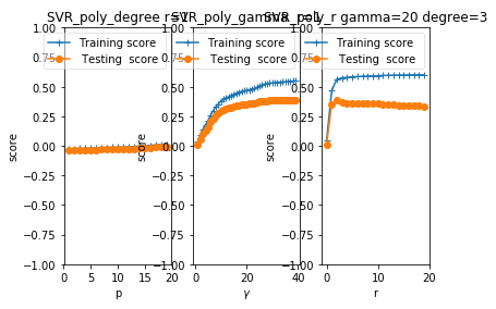
test_SVR_poly(X_train,X_test,y_train,y_test) 

def test_SVR_rbf(*data):
    '''
    测试 高斯核的 SVR 的预测性能随 gamma 参数的影响
    '''
    X_train,X_test,y_train,y_test=data
    gammas=range(1,20)
    train_scores=[]
    test_scores=[]
    for gamma in gammas:
        regr=svm.SVR(kernel='rbf',gamma=gamma)
        regr.fit(X_train,y_train)
        train_scores.append(regr.score(X_train,y_train))
        test_scores.append(regr.score(X_test, y_test))
    fig=plt.figure()
    ax=fig.add_subplot(1,1,1)
    ax.plot(gammas,train_scores,label="Training score ",marker='+' )
    ax.plot(gammas,test_scores,label= " Testing  score ",marker='o' )
    ax.set_title( "SVR_rbf")
    ax.set_xlabel(r"$\gamma$")
    ax.set_ylabel("score")
    ax.set_ylim(-1,1)
    ax.legend(loc="best",framealpha=0.5)
    plt.show()

# 调用 test_SVR_rbf
test_SVR_rbf(X_train,X_test,y_train,y_test) 

def test_SVR_sigmoid(*data):
    '''
    测试 sigmoid 核的 SVR 的预测性能随 gamma、coef0 的影响.
    '''
    X_train,X_test,y_train,y_test=data
    fig=plt.figure()

    ### 测试 gammam，固定 coef0 为 0.01 ####
    gammas=np.logspace(-1,3)
    train_scores=[]
    test_scores=[]

    for gamma in gammas:
        regr=svm.SVR(kernel='sigmoid',gamma=gamma,coef0=0.01)
        regr.fit(X_train,y_train)
        train_scores.append(regr.score(X_train,y_train))
        test_scores.append(regr.score(X_test, y_test))
    ax=fig.add_subplot(1,2,1)
    ax.plot(gammas,train_scores,label="Training score ",marker='+' )
    ax.plot(gammas,test_scores,label= " Testing  score ",marker='o' )
    ax.set_title( "SVR_sigmoid_gamma r=0.01")
    ax.set_xscale("log")
    ax.set_xlabel(r"$\gamma$")
    ax.set_ylabel("score")
    ax.set_ylim(-1,1)
    ax.legend(loc="best",framealpha=0.5)
    ### 测试 r ，固定 gamma 为 10 ######
    rs=np.linspace(0,5)
    train_scores=[]
    test_scores=[]

    for r in rs:
        regr=svm.SVR(kernel='sigmoid',coef0=r,gamma=10)
        regr.fit(X_train,y_train)
        train_scores.append(regr.score(X_train,y_train))
        test_scores.append(regr.score(X_test, y_test))
    ax=fig.add_subplot(1,2,2)
    ax.plot(rs,train_scores,label="Training score ",marker='+' )
    ax.plot(rs,test_scores,label= " Testing  score ",marker='o' )
    ax.set_title( "SVR_sigmoid_r gamma=10")
    ax.set_xlabel(r"r")
    ax.set_ylabel("score")
    ax.set_ylim(-1,1)
    ax.legend(loc="best",framealpha=0.5)
    plt.show()

# 调用 test_SVR_sigmoid
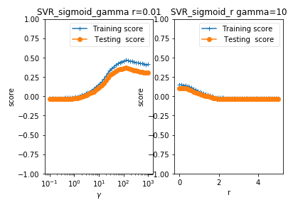
test_SVR_sigmoid(X_train,X_test,y_train,y_test)