终于成功仿了一次Kalman滤波器

终于成功仿了一次Kalman滤波器

首先是测试了从网上down的一段代码

% KALMANF - updates a system state vector estimate based upon an
% observation, using a discrete Kalman filter.
%
% Version 1.0, June 30, 2004
%
% This tutorial function was written by Michael C. Kleder
% (Comments are appreciated at: public@kleder.com)
%
% INTRODUCTION
%
% Many people have heard of Kalman filtering, but regard the topic
% as mysterious. While it's true that deriving the Kalman filter and
% proving mathematically that it is "optimal" under a variety of
% circumstances can be rather intense, applying the filter to
% a basic linear system is actually very easy. This Matlab file is
% intended to demonstrate that.
%
% An excellent paper on Kalman filtering at the introductory level,
% without detailing the mathematical underpinnings, is:
% "An Introduction to the Kalman Filter"
% Greg Welch and Gary Bishop, University of North Carolina
% http://www.cs.unc.edu/~welch/kalman/kalmanIntro.html
%
% PURPOSE:
%
% The purpose of each iteration of a Kalman filter is to update
% the estimate of the state vector of a system (and the covariance
% of that vector) based upon the information in a new observation.
% The version of the Kalman filter in this function assumes that
% observations occur at fixed discrete time intervals. Also, this
% function assumes a linear system, meaning that the time evolution
% of the state vector can be calculated by means of a state transition
% matrix.
%
% USAGE:
%
% s = kalmanf(s)
%
% "s" is a "system" struct containing various fields used as input
% and output. The state estimate "x" and its covariance "P" are
% updated by the function. The other fields describe the mechanics
% of the system and are left unchanged. A calling routine may change
% these other fields as needed if state dynamics are time-dependent;
% otherwise, they should be left alone after initial values are set.
% The exceptions are the observation vectro "z" and the input control
% (or forcing function) "u." If there is an input function, then
% "u" should be set to some nonzero value by the calling routine.
%
% SYSTEM DYNAMICS:
%
% The system evolves according to the following difference equations,
% where quantities are further defined below:
%
% x = Ax + Bu + w meaning the state vector x evolves during one time
% step by premultiplying by the "state transition
% matrix" A. There is optionally (if nonzero) an input
% vector u which affects the state linearly, and this
% linear effect on the state is represented by
% premultiplying by the "input matrix" B. There is also
% gaussian process noise w.
% z = Hx + v meaning the observation vector z is a linear function
% of the state vector, and this linear relationship is
% represented by premultiplication by "observation
% matrix" H. There is also gaussian measurement
% noise v.
% where w ~ N(0,Q) meaning w is gaussian noise with covariance Q
% v ~ N(0,R) meaning v is gaussian noise with covariance R
%
% VECTOR VARIABLES:
%
% s.x = state vector estimate. In the input struct, this is the
% "a priori" state estimate (prior to the addition of the
% information from the new observation). In the output struct,
% this is the "a posteriori" state estimate (after the new
% measurement information is included).
% s.z = observation vector
% s.u = input control vector, optional (defaults to zero).
%
% MATRIX VARIABLES:
%
% s.A = state transition matrix (defaults to identity).
% s.P = covariance of the state vector estimate. In the input struct,
% this is "a priori," and in the output it is "a posteriori."
% (required unless autoinitializing as described below).
% s.B = input matrix, optional (defaults to zero).
% s.Q = process noise covariance (defaults to zero).
% s.R = measurement noise covariance (required).
% s.H = observation matrix (defaults to identity).
%
% NORMAL OPERATION:
%
% (1) define all state definition fields: A,B,H,Q,R
% (2) define intial state estimate: x,P
% (3) obtain observation and control vectors: z,u
% (4) call the filter to obtain updated state estimate: x,P
% (5) return to step (3) and repeat
%
% INITIALIZATION:
%
% If an initial state estimate is unavailable, it can be obtained
% from the first observation as follows, provided that there are the
% same number of observable variables as state variables. This "auto-
% intitialization" is done automatically if s.x is absent or NaN.
%
%x = inv(H)*z
%P = inv(H)*R*inv(H')
%
% This is mathematically equivalent to setting the initial state estimate
% covariance to infinity.
%
% SCALAR EXAMPLE (Automobile Voltimeter):
%
% % Define the system as a constant of 12 volts:
function T
clear s
s.x = 12;
s.A = 1;
% % Define a process noise (stdev) of 2 volts as the car operates:
s.Q = 2^2; % variance, hence stdev^2
% Define the voltimeter to measure the voltage itself:
s.H = 1;
% % Define a measurement error (stdev) of 2 volts:
s.R = 2^2; % variance, hence stdev^2
%Do not define any system input (control) functions:
s.B = 0;
s.u = 0;
% % Do not specify an initial state:
s.x = nan;
s.P = nan;
% % Generate random voltages and watch the filter operate.
tru=[]; % truth voltage
for t=1:20
    tru(end+1) = randn*2+12;
    s(end).z = tru(end) + randn*2; % create a measurement
    s(end+1)=kalmanf(s(end)); % perform a Kalman filter iteration
    % end
    % figure
    % hold on
    % grid on
    % % plot measurement data:
    hz=plot([s(1:end-1).z],'r');hold on
    % % plot a-posteriori state estimates:
    hk=plot([s(2:end).x],'b-');hold on
    ht=plot(tru,'g-');hold on
    legend('observations','Kalman output','true voltage',0)
    title('Automobile Voltimeter Example')
    % hold off
end    
    
function s = kalmanf(s)

% set defaults for absent fields:
if ~isfield(s,'x'); s.x=nan*z; end
if ~isfield(s,'P'); s.P=nan; end
if ~isfield(s,'z'); error('Observation vector missing'); end
if ~isfield(s,'u'); s.u=0; end
if ~isfield(s,'A'); s.A=eye(length(x)); end
if ~isfield(s,'B'); s.B=0; end
if ~isfield(s,'Q'); s.Q=zeros(length(x)); end
if ~isfield(s,'R'); error('Observation covariance missing'); end
if ~isfield(s,'H'); s.H=eye(length(x)); end

if isnan(s.x)
    % initialize state estimate from first observation
    if diff(size(s.H))
        error('Observation matrix must be square and invertible for state autointialization.');
    end
    s.x = inv(s.H)*s.z;
    s.P = inv(s.H)*s.R*inv(s.H'); 
else
    
    % This is the code which implements the discrete Kalman filter:
    
    % Prediction for state vector and covariance:
    s.x = s.A*s.x + s.B*s.u;
    s.P = s.A * s.P * s.A' + s.Q;
    
    % Compute Kalman gain factor:
    K = s.P*s.H'*inv(s.H*s.P*s.H'+s.R);
    
    % Correction based on observation:
    s.x = s.x + K*(s.z-s.H*s.x);
    s.P = s.P - K*s.H*s.P;
    
    % Note that the desired result, which is an improved estimate
    % of the sytem state vector x and its covariance P, was obtained
    % in only five lines of code, once the system was defined. (That's
    % how simple the discrete Kalman filter is to use.) Later,
    % we'll discuss how to deal with nonlinear systems.
    
end

后来不过瘾，自己写了一个，没想到稍微改了一改竟然成功了，效果还不错

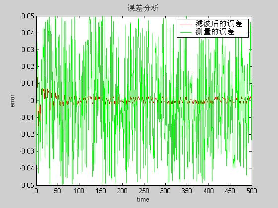
% 状态
% xk=A•xk-1+B•uk+wk
% zk=H•xk+vk,
% p(w) ~ N(0,Q)
% p(v) ~ N(0,R),

% 预测
% x'k=A•xk+B•uk
% P'k=A•P(k-1)*AT + Q
% 修正
% Kk=P'k•HT•(H•P'k•HT+R)-1
% xk=x'k+Kk•(zk-H•x'k)
% Pk=(I-Kk•H)•P'k

%要注意的是：必须把系统状态和kalman滤波器内部预测的状态分开
function Test
A=[1 0.1;0 1];
B=0;
Xp=rand(2,1)*0.1; 
X=[0 0]';
H=[1 0];
Q=eye(2)*1e-5;
R=eye(1)*0.1; 
P=eye(2);% P'(k)
angle=[];
angle_m=[];
angle_real=[];
for i=1:500
    angle_real=[angle_real X(1)]; %实际角度
    
    [Xp,P]=Predict(A,Xp,P,Q); 
    
    X=A*X+rand(2,1)*1e-5;
    z_m=H*X+rand(1,1)*0.1-0.05;  
    angle_m=[angle_m z_m(1)];   %测量的角度
        
    [Xp,P]=Correct(P,H,R,X,z_m);
    angle=[angle Xp(1)];     %预测的角度    
end
t=1:500;
plot(t,angle,'r',t,angle_m,'g',t,angle_real,'b')
legend('预测值','测量值','实际值')

figure
plot(t,angle-angle_real,'r',t,angle_m-angle_real,'g')
legend('滤波后的误差','测量的误差')
title('误差分析')
xlabel('time');
ylabel('error');

function [Xk,Pk]=Predict(A,Xk,Pk_1,Q)
Xk=A*Xk;
Pk=A*Pk_1*A'+Q;

function [Xk,Pk]=Correct(Pk,H,R,Xk,zk)
Kk=Pk * H' * inv(H * Pk * H' + R);
Xk=Xk+ Kk*(zk-H*Xk);
Pk=(eye(size(Pk,1)) - Kk*H)*Pk;

 

 

顺便附上几张仿真图
这是状态图

这是误差分析