快速入门pandas进行数据挖掘数据分析[多维度排序、数据筛选、分组计算、透视表](一)
1. 快速入门python,python基本语法
Python使用缩进(tab或者空格)来组织代码,而不是像其 他语言比如R、C++、Java和Perl那样用大括号。考虑使用for循 环来实现排序算法:
for x in list_values:

if x < 10:

small.append(x)

else:

bigger.append(x)
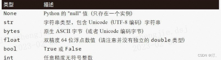
标量类型
2.3,4,null,True都是标量
变量
a=2

b='this is alibaba'

c=[1,2,456.,np.nan,c]
数据结构
#列表(list)

myList=[1,2,"hello bro",np.nan,3456225.0987]

#元组(tuple,不可修改)

myTuple=(2,3,'hey morning!',89,np.nan)

#字典(dictionary,俗称键值对)

myDictionary={'key1' :23, "key2" : "hahahh,哈哈哈", "key3" : 78}

#集合(set,集合)

myset=set({'happy','sad','sad'})
运算
a=8

b=2

c=a**b

d=a/b

d
函数(打包好的功能块)
#定义一个计算平均数的函数

def get_avg(values):

if len(values) == 0:#如果输入的list没有值

return 0 #返回0

sum_v = 0

#遍历所有值

for value in values:

#前一个和加上后一个值

sum_v = value+sum_v

return sum_v / len(values)

avg = get_avg([1, 2, 3, 4])

avg
def get_avg(values):

if len(values) == 0:#如果输入的list没有值

return 0 #返回0

sum_v = 0

#遍历所有值

for value in values:

#前一个和加上后一个值

sum_v = value+sum_v

return sum_v / len(values)

avg = get_avg([1, 2, 3, 4])

avg
循环
sum10 = 0

for i in range(1, 11):

sum10 = sum10+i

print(sum10)
sum10 = 0

for i in range(1, 11):

sum10 = sum10+i

print(i)

print(sum10)
2. 快速入门pandas
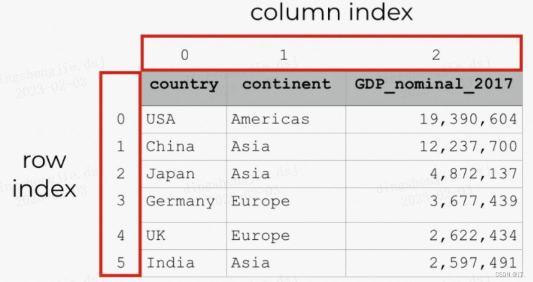
2.1 pandas核心数据结构和常用API
pandas资料下载链接:https://download.csdn.net/download/sinat_39620217/87413329


2.2 pandas 基础数据操作
导入常用的数据分析库
import numpy as np

import pandas as pd

#创建一个series

s = pd.Series([1, 3, 5, np.nan, 6, 8])

s

0 1.0

1 3.0

2 5.0

3 NaN

4 6.0

5 8.0

dtype: float64
#创建一个时间序列

dates = pd.date_range("20130101", periods=6)

dates

DatetimeIndex(['2023-02-03', '2023-02-04', '2023-02-05', '2023-02-06',

'2023-02-07', '2023-02-08'],

dtype='datetime64[ns]', freq='D')
#以时间序列为index,以“ABCD”为列明,用24个符合正态分布的随机数作为数值

df = pd.DataFrame(np.random.randn(6, 4), index=dates, columns=list("ABCD"))

df

A B C D

2023-02-03 -1.688539 -0.687145 -0.087825 -0.113740

2023-02-04 -0.483402 -2.333871 -1.078778 1.786806

2023-02-05 1.154374 0.976104 0.004643 0.754242

2023-02-06 -0.005039 -0.170111 0.578378 0.604114

2023-02-07 1.923344 -1.132254 1.408248 0.101545

2023-02-08 0.876144 1.589423 1.678817 -1.271310
#另一种创建df的方法

df2 = pd.DataFrame(

{

"A": 1.0,

"B": pd.Timestamp("20130102"),

"C": pd.Series(1, index=list(range(4)), dtype="float32"),

"D": np.array([3] * 4, dtype="int32"),

"E": pd.Categorical(["test", "train", "test", "train"]),

"F": "foo",

}

)

df2

A B C D E F

0 1.0 2013-01-02 1.0 3 test foo

1 1.0 2013-01-02 1.0 3 train foo

2 1.0 2013-01-02 1.0 3 test foo

3 1.0 2013-01-02 1.0 3 train foo
#看下数据类型

df2.dtypes

A float64

B datetime64[ns]

C float32

D int32

E category

F object

dtype: object

df2.head(2)

df2.tail()

df2.sample(3)

A B C D E F

0 1.0 2013-01-02 1.0 3 test foo

1 1.0 2013-01-02 1.0 3 train foo

A B C D E F

0 1.0 2013-01-02 1.0 3 test foo

1 1.0 2013-01-02 1.0 3 train foo

2 1.0 2013-01-02 1.0 3 test foo

3 1.0 2013-01-02 1.0 3 train foo

A B C D E F

1 1.0 2013-01-02 1.0 3 train foo

2 1.0 2013-01-02 1.0 3 test foo

0 1.0 2013-01-02 1.0 3 test foo
#导入本地数据到python内存

diamonds_df=pd.read_csv('data/diamonds.csv')

diamonds_df

carat cut color clarity depth table price x y z

0 0.23 Ideal E SI2 61.5 55.0 326 3.95 3.98 2.43

1 0.21 Premium E SI1 59.8 61.0 326 3.89 3.84 2.31

2 0.23 Good E VS1 56.9 65.0 327 4.05 4.07 2.31

3 0.29 Premium I VS2 62.4 58.0 334 4.20 4.23 2.63

4 0.31 Good J SI2 63.3 58.0 335 4.34 4.35 2.75

... ... ... ... ... ... ... ... ... ... ...

53935 0.72 Ideal D SI1 60.8 57.0 2757 5.75 5.76 3.50

53936 0.72 Good D SI1 63.1 55.0 2757 5.69 5.75 3.61

53937 0.70 Very Good D SI1 62.8 60.0 2757 5.66 5.68 3.56

53938 0.86 Premium H SI2 61.0 58.0 2757 6.15 6.12 3.74

53939 0.75 Ideal D SI2 62.2 55.0 2757 5.83 5.87 3.64

53940 rows × 10 columns
#查看数据的信息或者基本情况

diamonds_df.info()

<class 'pandas.core.frame.DataFrame'>

RangeIndex: 53940 entries, 0 to 53939

Data columns (total 10 columns):

# Column Non-Null Count Dtype

--- ------ -------------- -----

0 carat 53940 non-null float64

1 cut 53940 non-null object

2 color 53940 non-null object

3 clarity 53940 non-null object

4 depth 53940 non-null float64

5 table 53940 non-null float64

6 price 53940 non-null int64

7 x 53940 non-null float64

8 y 53940 non-null float64

9 z 53940 non-null float64

dtypes: float64(6), int64(1), object(3)

memory usage: 4.1+ MB

#查看索引

diamonds_df.index

RangeIndex(start=0, stop=53940, step=1)

#查看列名

diamonds_df.columns

Index(['carat', 'cut', 'color', 'clarity', 'depth', 'table', 'price', 'x', 'y',

'z'],

dtype='object')
#查看数据基本情况

diamonds_df.describe()

carat depth table price x y z

count 53940.000000 53940.000000 53940.000000 53940.000000 53940.000000 53940.000000 53940.000000

mean 0.797940 61.749405 57.457184 3932.799722 5.731157 5.734526 3.538734

std 0.474011 1.432621 2.234491 3989.439738 1.121761 1.142135 0.705699

min 0.200000 43.000000 43.000000 326.000000 0.000000 0.000000 0.000000

25% 0.400000 61.000000 56.000000 950.000000 4.710000 4.720000 2.910000

50% 0.700000 61.800000 57.000000 2401.000000 5.700000 5.710000 3.530000

75% 1.040000 62.500000 59.000000 5324.250000 6.540000 6.540000 4.040000

max 5.010000 79.000000 95.000000 18823.000000 10.740000 58.900000 31.800000

#行列转换

df.T

2023-02-03 2023-02-04 2023-02-05 2023-02-06 2023-02-07 2023-02-08

A -1.688539 -0.483402 1.154374 -0.005039 1.923344 0.876144

B -0.687145 -2.333871 0.976104 -0.170111 -1.132254 1.589423

C -0.087825 -1.078778 0.004643 0.578378 1.408248 1.678817

D -0.113740 1.786806 0.754242 0.604114 0.101545 -1.271310
2.3 pandas多维度排序
#对数据进行排序

df.sort_values(by="B",ascending=False)

diamonds_df.head()

A B C D

2023-02-08 0.876144 1.589423 1.678817 -1.271310

2023-02-05 1.154374 0.976104 0.004643 0.754242

2023-02-06 -0.005039 -0.170111 0.578378 0.604114

2023-02-03 -1.688539 -0.687145 -0.087825 -0.113740

2023-02-07 1.923344 -1.132254 1.408248 0.101545

2023-02-04 -0.483402 -2.333871 -1.078778 1.786806
#按照cut和color联合排序

diamonds_df.sort_values(by=['cut','color','price'],ascending=False)

carat cut color clarity depth table price x y z

27586 2.44 Very Good J VS2 58.1 60.0 18430 8.89 8.93 5.18

27352 2.39 Very Good J VS1 59.6 60.0 17920 8.71 8.77 5.21

27185 2.44 Very Good J SI1 62.9 53.0 17472 8.58 8.62 5.41

27024 2.74 Very Good J SI2 61.5 62.0 17164 8.87 8.90 5.46

26958 2.50 Very Good J SI1 62.8 57.0 17028 8.58 8.65 5.41

... ... ... ... ... ... ... ... ... ... ...

28534 0.42 Fair D SI1 64.7 61.0 675 4.70 4.73 3.05

25695 0.40 Fair D SI1 65.1 55.0 644 4.63 4.68 3.03

10380 0.29 Fair D VS2 64.7 62.0 592 4.14 4.11 2.67

2711 0.25 Fair D VS1 61.2 55.0 563 4.09 4.11 2.51

48630 0.30 Fair D SI2 64.6 54.0 536 4.29 4.25 2.76

53940 rows × 10 columns
2.4 pandas数据筛选
#列范围

diamonds_df[["cut","depth","price"]]

cut depth price

0 Ideal 61.5 326

1 Premium 59.8 326

2 Good 56.9 327

3 Premium 62.4 334

4 Good 63.3 335
#行范围

diamonds_df[6:9]

carat cut color clarity depth table price x y z

6 0.24 Very Good I VVS1 62.3 57.0 336 3.95 3.98 2.47

7 0.26 Very Good H SI1 61.9 55.0 337 4.07 4.11 2.53

8 0.22 Fair E VS2 65.1 61.0 337 3.87 3.78 2.49
#按行范围和列具体

diamonds_df.loc[5:9, ["carat","price","x"]]

carat price x

5 0.24 336 3.94

6 0.24 336 3.95

7 0.26 337 4.07

8 0.22 337 3.87

9 0.23 338 4.00
#按行具体和列范围

#注意:具体必须要用list来承载(中括号),范围不能用中括号

diamonds_df.loc[[3,6,9], "cut":"price"]

cut color clarity depth table price

3 Premium I VS2 62.4 58.0 334

6 Very Good I VVS1 62.3 57.0 336

9 Very Good H VS1 59.4 61.0 338
#按行逻辑和列范围

diamonds_df.loc[diamonds_df.carat>0.3, ["carat","price"]]

carat price

4 0.31 335

13 0.31 344

15 0.32 345

23 0.31 353

24 0.31 353

... ... ...
#按条件筛选

#按照某列进行筛选

diamonds_df[(diamonds_df["carat"] > 0.3) & (diamonds_df["price"] < 400)]

carat cut color clarity depth table price x y z

4 0.31 Good J SI2 63.3 58.0 335 4.34 4.35 2.75

13 0.31 Ideal J SI2 62.2 54.0 344 4.35 4.37 2.71

15 0.32 Premium E I1 60.9 58.0 345 4.38 4.42 2.68

23 0.31 Very Good J SI1 59.4 62.0 353 4.39 4.43 2.62

24 0.31 Very Good J SI1 58.1 62.0 353 4.44 4.47 2.59

28271 0.32 Good D I1 64.0 54.0 361 4.33 4.36 2.78

28277 0.31 Very Good J SI1 61.9 59.0 363 4.28 4.32 2.66

28278 0.31 Very Good J SI1 62.7 59.0 363 4.29 4.32 2.70

28279 0.31 Premium J SI1 60.9 60.0 363 4.36 4.38 2.66

28280 0.31 Good J SI1 63.5 55.0 363 4.30 4.33 2.74
#筛选cut属于Premium和Good

diamonds_df[(diamonds_df['cut'].isin(['Premium','Good'])) &

(diamonds_df['carat']>0.3) & (diamonds_df['price']<400) ]

carat cut color clarity depth table price x y z

4 0.31 Good J SI2 63.3 58.0 335 4.34 4.35 2.75

15 0.32 Premium E I1 60.9 58.0 345 4.38 4.42 2.68

28271 0.32 Good D I1 64.0 54.0 361 4.33 4.36 2.78

28279 0.31 Premium J SI1 60.9 60.0 363 4.36 4.38 2.66

28280 0.31 Good J SI1 63.5 55.0 363 4.30 4.33 2.74

28284 0.32 Premium J SI1 62.2 59.0 365 4.37 4.41 2.73

34928 0.32 Good J SI1 63.2 56.0 374 4.31 4.36 2.74

34929 0.32 Good I SI2 63.4 56.0 374 4.34 4.37 2.76

34932 0.32 Good I SI2 63.1 58.0 374 4.34 4.41 2.76

34939 0.31 Good I SI1 64.3 55.0 377 4.27 4.29 2.75
2.5 pandas分组计算
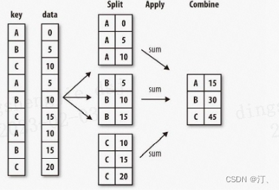
#分组计算

df = pd.DataFrame(

{

"A": ["foo", "bar", "foo", "bar", "foo", "bar", "foo", "foo"],

"B": ["one", "one", "two", "three", "two", "two", "one", "three"],

"C": np.random.randn(8),

"D": np.random.randn(8),

}

)

df

A B C D

0 foo one -1.265302 -1.718949

1 bar one -0.814010 0.097433

2 foo two -1.359590 0.708358

3 bar three 0.562501 -2.525745

4 foo two 1.036076 0.455022

5 bar two 2.192717 -0.163239

6 foo one 0.623262 -0.632277

7 foo three -0.791469 1.801869
#按照A分组,分别计算C和D的和

df.groupby("A")[["C", "D"]].sum()

C D

A

bar 1.941208 -2.591551

foo -1.757023 0.614024
#按照多列进行分组计算

df.groupby(["A", "B"]).sum()

C D

A B

bar one -0.814010 0.097433

three 0.562501 -2.525745

two 2.192717 -0.163239

foo one -0.642040 -2.351226

three -0.791469 1.801869

two -0.323514 1.163381
#按照cut和color的组合计算平均价格

diamonds_df.groupby(by=['cut','color'])[['price']].mean().round(2).reset_index()

cut color price

0 Fair D 4291.06

1 Fair E 3682.31

2 Fair F 3827.00

3 Fair G 4239.25

4 Fair H 5135.68

5 Fair I 4685.45

6 Fair J 4975.66

7 Good D 3405.38

8 Good E 3423.64

9 Good F 3495.75

10 Good G 4123.48

11 Good H 4276.25

12 Good I 5078.53

13 Good J 4574.17
2.6 pandas透视表
#透视表

df = pd.DataFrame(

{

"甲": ["one", "one", "two", "three"] * 3,

"乙": ["A", "B", "C"] * 4,

"丙": ["foo", "foo", "foo", "bar", "bar", "bar"] * 2,

"D": np.random.randn(12),

"E": np.random.randn(12),

}

)

df

甲 乙 丙 D E

0 one A foo 0.593815 0.399765

1 one B foo 0.943989 -0.073500

2 two C foo 0.504724 0.916902

3 three A bar 1.377307 0.930002

4 one B bar 0.364403 2.430547

5 one C bar -0.392653 -0.307336

6 two A foo -0.698488 2.202757

7 three B foo -2.046343 0.562993

8 one C foo -0.570906 0.719652

9 one A bar -1.493323 0.612229

10 two B bar 1.744241 0.616304

11 three C bar 2.337644 1.568032
pd.pivot_table(df, values="D", index=["甲","乙"], columns=["丙"],aggfunc='mean')

丙 bar foo

甲 乙

one A -1.493323 0.593815

B 0.364403 0.943989

C -0.392653 -0.570906

three A 1.377307 NaN

B NaN -2.046343

C 2.337644 NaN

two A NaN -0.698488

B 1.744241 NaN

C NaN 0.504724
快速入门pandas进行数据挖掘数据分析[多维度排序、数据筛选、分组计算、透视表](一)的更多相关文章
- 快速入门Pandas
教你十分钟学会使用pandas. pandas是python数据分析的一个最重要的工具. 基本使用 # 一般以pd作为pandas的缩写 import pandas as pd # 读取文件 df = ...
- 快速入门 Pandas
先po几个比较好的Pandas入门网站十分钟入门:http://www.codingpy.com/article/a-quick-intro-to-pandas/手册前2章:http://pda.re ...
- Hawk 1.2 快速入门2 (大众点评18万美食数据)
本文将讲解通过本软件,获取大众点评的所有美食数据,可选择任一城市,也可以很方便地修改成获取其他生活门类信息的爬虫. 本文将省略原理,一步步地介绍如何在20分钟内完成爬虫的设计,基本不需要编程,还能自动 ...
- pyhton中pandas数据分析模块快速入门(非常容易懂)
//2019.07.16python中pandas模块应用1.pandas是python进行数据分析的数据分析库,它提供了对于大量数据进行分析的函数库和各种方法,它的官网是http://pandas. ...
- 小白学 Python 数据分析(12):Pandas (十一)数据透视表(pivot_table)
人生苦短,我用 Python 前文传送门: 小白学 Python 数据分析(1):数据分析基础 小白学 Python 数据分析(2):Pandas (一)概述 小白学 Python 数据分析(3):P ...
- python库学习笔记——分组计算利器:pandas中的groupby技术
最近处理数据需要分组计算,又用到了groupby函数,温故而知新. 分组运算的第一阶段,pandas 对象(无论是 Series.DataFrame 还是其他的)中的数据会根据你所提供的一个或多个键被 ...
- pandas快速入门
pandas快速入门 numpy之后让我们紧接着学习pandas.Pandas最初被作为金融数据分析工具而开发出来,后来因为其强大性以及友好性,在数据分析领域被广泛使用,下面让我们一窥究竟. 本文参考 ...
- Python pandas快速入门
Python pandas快速入门2017年03月14日 17:17:52 青盏 阅读数:14292 标签: python numpy 数据分析 更多 个人分类: machine learning 来 ...
- Pandas 快速入门(二)
本文的例子需要一些特殊设置,具体可以参考 Pandas快速入门(一) 数据清理和转换 我们在进行数据处理时,拿到的数据可能不符合我们的要求.有很多种情况,包括部分数据缺失,一些数据的格式不正确,一些数 ...
- python快速入门——进入数据挖掘你该有的基础知识
这篇文章是用来总结python中重要的语法,通过这些了解你可以快速了解一段python代码的含义 Python 的基础语法来带你快速入门 Python 语言.如果你想对 Python 有全面的了解请关 ...
随机推荐
- 三、Ocelot请求聚合与负载均衡
上一篇文章介绍了在.Net Core中如何使用Ocelot:https://www.cnblogs.com/yangleiyu/p/16847439.html 本文介绍在ocelot的请求聚合与负载均 ...
- Django开发汇总
基本配置 # 设置数据库为使用的mysql DATABASES = { 'default': { 'ENGINE': 'django.db.backends.mysql', 'NAME': 'libr ...
- Git创建、diff代码、回退版本、撤回代码,学废了吗
.eye-care { background-color: rgba(199, 237, 204, 1); padding: 10px } .head-box { display: flex } .t ...
- MySQL数据库的性能分析 ---图书《软件性能测试分析与调优实践之路》-手稿节选
1 .MySQL数据库的性能监控 1.1.如何查看MySQL数据库的连接数 连接数是指用户已经创建多少个连接,也就是MySQL中通过执行 SHOW PROCESSLIST命令输出结果中运行着的线程 ...
- [CS61A] Lecture 4. Higher-Order Functions & Project 1: The Game of Hog
[CS61A] Lecture 4. Higher-Order Functions & Project 1: The Game of Hog Lecture Lecture 4. Higher ...
- ROSIntegration ROSIntegrationVision与虚幻引擎4(Unreal Engine 4)的配置
ROSIntegration ROSIntegrationVision与虚幻引擎4(Unreal Engine 4)的配置 操作系统:Ubuntu 18.04 虚幻引擎:4.26.2 目录 ROSIn ...
- windows10熄屏断网问题解决
以前用windowsserver的操作系统可以随时随地的远程,最近因工作需要安装了一个windows10的远程设备,发现windows10系统长时间未使用便连不上了,远程不了,ping不通,本地连接断 ...
- npm安装hexo报错
报错提示 npm WARN saveError ENOENT: no such file or directory, open '/home/linux1/package.json' npm noti ...
- 总算给女盆友讲明白了,如何使用stream流的filter()操作
一.引言 在上一篇文章中<这么简单,还不会使用java8 stream流的map()方法吗?>分享了使用stream的map()方法,不知道小伙伴还有印象吗,先来回顾下要点,map()方法 ...
- 【Java SE】Day10接口、多态
一.接口 1.概述 是一种引用类型,是方法的集合,内部封装了各种方法 引用类型:数组.类.接口.包装类 2.方法的定义格式 抽象方法:无方法体,子类实现 默认方法: 静态方法:static修饰,可以由 ...