week3编程作业: Logistic Regression中一些难点的解读

%% ============ Part : Compute Cost and Gradient ============
%  In this part of the exercise, you will implement the cost and gradient
%  for logistic regression. You neeed to complete the code in
%  costFunction.m

%  Setup the data matrix appropriately, and add ones for the intercept term
[m, n] = size(X);

% Add intercept term to x and X_test
X = [ones(m, ) X];

% Initialize fitting parameters
initial_theta = zeros(n + , );

% Compute and display initial cost and gradient
[cost, grad] = costFunction(initial_theta, X, y);

难点1：X和theta的维度变化，怎么变得，为什么？

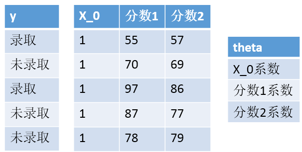
X加了一列1，θ加了一行θ₀,因为最后边界是θ₀+θ₁X₁+θ₂X₂,要符合矩阵运算

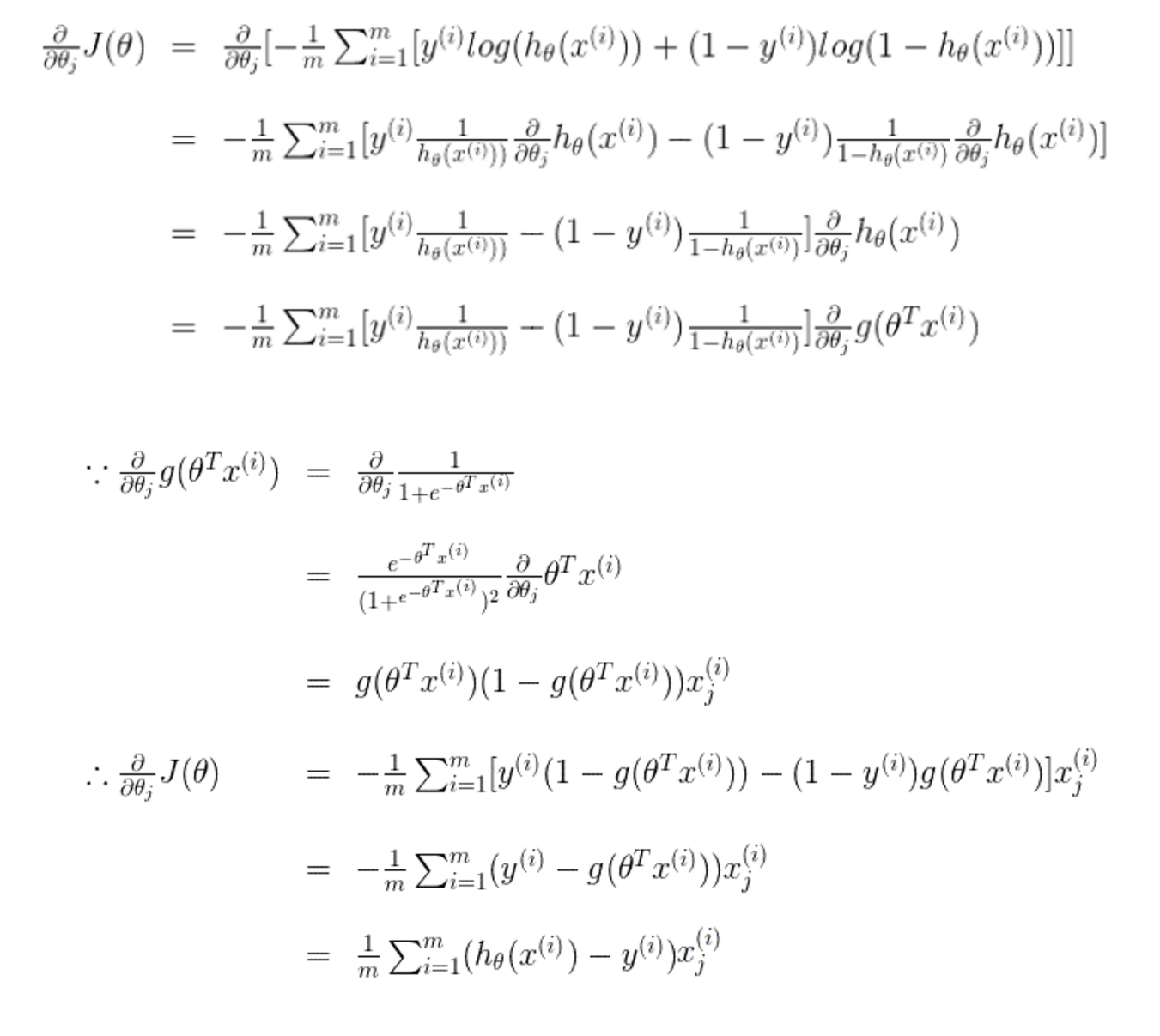
难点2：costFunction中grad是什么函数，有什么作用？

w.r.t 什么意思？

with regard to
with reference to

关于的意思

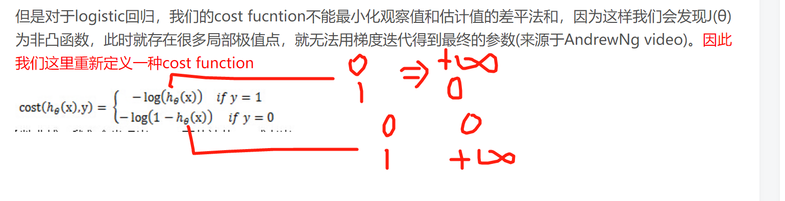
难点3：linear regression的代价函数和logistic regression的代价函数，为什么不一样？

和幂次有关，如果还用原来的代价函数，那么会有很多局部最值，没有办法梯度下降到最小值。

另一个解读角度：从最大似然函数出发考虑。

下面的文章写得很好，参考链接：

　　　 http://blog.csdn.net/lu597203933/article/details/38468303

http://blog.csdn.net/it_vitamin/article/details/45625143

%% ============= Part : Optimizing using fminunc  =============
%  In this exercise, you will use a built-in function (fminunc) to find the
%  optimal parameters theta.

%  Set options for fminunc
options = optimset('GradObj', 'on', 'MaxIter', );

%  Run fminunc to obtain the optimal theta
%  This function will return theta and the cost
[theta, cost] = ...
    fminunc(@(t)(costFunction(t, X, y)), initial_theta, options);

难点4：optimset是什么作用？

options = optimset('GradObj', 'on', 'MaxIter', 400); //

通过optimset函数设置或改变这些参数。其中有的参数适用于所有的优化算法，有的则只适用于大型优化问题，另外一些则只适用于中型问题。

LargeScale – 当设为'on'时使用大型算法，若设为'off'则使用中型问题的算法。
      适用于大型和中型算法的参数：
Diagnostics – 打印最小化函数的诊断信息。
Display – 显示水平。选择'off'，不显示输出；选择'iter'，显示每一步迭代过程的输出；选择'final'，显示最终结果。打印最小化函数的诊断信息。
GradObj – 用户定义的目标函数的梯度。对于大型问题此参数是必选的，对于中型问题则是可选项。
MaxFunEvals – 函数评价的最大次数。
MaxIter – 最大允许迭代次数。
TolFun – 函数值的终止容限。
TolX – x处的终止容限。

options = optimset('param1',value1,'param2',value2,...) %设置所有参数及其值，未设置的为默认值

options = optimset('GradObj', 'on', 'MaxIter', 400);

在使用options的函数中，参数是由用户自行定义的，最大递归次数为400

难点5：[theta, cost] = fminunc(@(t)(costFunction(t, X, y)), initial_theta, options)是怎么实现功能？

关于句柄@，参考偏文章：http://blog.csdn.net/gzp444280620/article/details/49252491

关于fiminuc,参考这篇文章：http://blog.csdn.net/gzp444280620/article/details/49272977

fminunc(@(t)(costFunction(t, X, y)), initial_theta, options);    %是为了当代码里面有这样的函数的时候，fminunc(1,θ，option)第一个参数，

会传递给costFunction(t, X, y)的第一个参数里面进行计算。

function plotDecisionBoundary(theta, X, y)
%PLOTDECISIONBOUNDARY Plots the data points X and y into a new figure with
%the decision boundary defined by theta
%   PLOTDECISIONBOUNDARY(theta, X,y) plots the data points with + for the
%   positive examples and o for the negative examples. X is assumed to be
%   a either
%   ) Mx3 matrix, where the first column is an all-ones column for the
%      intercept.
%   ) MxN, N> matrix, where the first column is all-ones

% Plot Data
plotData(X(:,:), y);
hold on

if size(X, ) <=
    % Only need  points to define a line, so choose two endpoints
    plot_x = [min(X(:,))-,  max(X(:,))+];

    % Calculate the decision boundary line//令theta装置乘以X等于0，即可

   plot_y = (-./theta()).*(theta().*plot_x + theta());

    % Plot, and adjust axes for better viewing
    plot(plot_x, plot_y)

    % Legend, specific for the exercise
    legend('Admitted', 'Not admitted', 'Decision Boundary')
    axis([, , , ])
else
    % Here is the grid range
    u = linspace(-, 1.5, );
    v = linspace(-, 1.5, );

    z = zeros(length(u), length(v));
    % Evaluate z = theta*x over the grid
    for i = :length(u)
        for j = :length(v)
            z(i,j) = mapFeature(u(i), v(j))*theta;
        end
    end
    z = z'; % important to transpose z before calling contour

    % Plot z =
    % Notice you need to specify the range [, ]
    contour(u, v, z, [, ], 'LineWidth', )
end
hold off

end

难点6：这个plotDecisionBoundary函数是怎么画出边界的？

plotDecisionBoundary中的下面的两行看不懂：

plot_x = [min(X(:,2))-2,  max(X(:,2))+2];  //直线的参数其实已经得到，选划线的范围，把直线画出来即可。为了美观，扩大了两个单位

% Calculate the decision boundary line//令theta装置乘以X等于0，即可 plot_y = (-1./theta(3)).*(theta(2).*plot_x + theta(1));

plot_y = (-1./theta(3)).*(theta(2).*plot_x + theta(1));

function plotData(X, y)    //会按照真类和假类分类 画出输入的点
%PLOTDATA Plots the data points X and y into a new figure
%   PLOTDATA(x,y) plots the data points with + for the positive examples
%   and o for the negative examples. X is assumed to be a Mx2 matrix.

% Create New Figure
figure; hold on;

% ====================== YOUR CODE HERE ======================
% Instructions: Plot the positive and negative examples on a
%               2D plot, using the option 'k+' for the positive
%               examples and 'ko' for the negative examples.
%
% Find Indices of Positive and Negative Examples              //返回 y=1和y=0的位置，也就是行数
  pos = find(y==);        neg = find(y == );                //利用find的查找功能，把正类和负类分开，并把横纵坐标保存在pos里面
% Plot Examples
plot(X(pos, ), X(pos, ), 'k+','LineWidth', , ...
'MarkerSize', );
plot(X(neg, ), X(neg, ), 'ko', 'MarkerFaceColor', 'y', ...
'MarkerSize', );

% =========================================================================

hold off;

end

%% =========== Part : Regularized Logistic Regression ============
%  In this part, you are given a dataset with data points that are not
%  linearly separable. However, you would still like to use logistic
%  regression to classify the data points.
%
%  To do so, you introduce more features to use -- in particular, you add
%  polynomial features to our data matrix (similar to polynomial
%  regression).
%

% Add Polynomial Features

% Note that mapFeature also adds a column of ones for us, so the intercept
% term is handled
X = mapFeature(X(:,), X(:,));

% Initialize fitting parameters
initial_theta = zeros(size(X, ), );

% Set regularization parameter lambda to
lambda = ;

% Compute and display initial cost and gradient for regularized logistic
% regression
[cost, grad] = costFunctionReg(initial_theta, X, y, lambda);

难点7：mapFeature是怎么工作的，原理？

难点8：[cost, grad] = costFunctionReg(initial_theta, X, y, lambda);怎么工作？

%% ============= Part : Regularization and Accuracies =============
%  Optional Exercise:
%  In this part, you will get to try different values of lambda and
%  see how regularization affects the decision coundart
%
%  Try the following values of lambda (, , , ).
%
%  How does the decision boundary change when you vary lambda? How does
%  the training set accuracy vary?
%

% Initialize fitting parameters
initial_theta = zeros(size(X, ), );

% Set regularization parameter lambda to  (you should vary this)
lambda = ;

% Set Options
options = optimset('GradObj', 'on', 'MaxIter', );

% Optimize
[theta, J, exit_flag] = ...
    fminunc(@(t)(costFunctionReg(t, X, y, lambda)), initial_theta, options);

难点9：为什么fminunc可以返回三个变量？

ps:先把问题记录一下，稍后会一个个解决。