（转）RL — Policy Gradient Explained

RL — Policy Gradient Explained

2019-05-02 21:12:57

This blog is copied from: https://medium.com/@jonathan_hui/rl-policy-gradients-explained-9b13b688b146

Photo by Alex Read

Policy Gradient Methods (PG) are frequently used algorithms in reinforcement learning (RL). The principle is very simple.

We observe and act.

A human takes actions based on observations. As a quote from Stephen Curry:

You have to rely on the fact that you put the work in to create the muscle memory and then trust that it will kick in. The reason you practice and work on it so much is so that during the game your instincts take over to a point where it feels weird if you don’t do it the right way.

 

Source

Constant practice is the key to build muscle memory for athletes. For PG, we train a policy to act based on observations. The training in PG makes actions with high rewards more likely, or vice versa.

We keep what is working and throw away what is not.

In policy gradients, Curry is our agent.

 

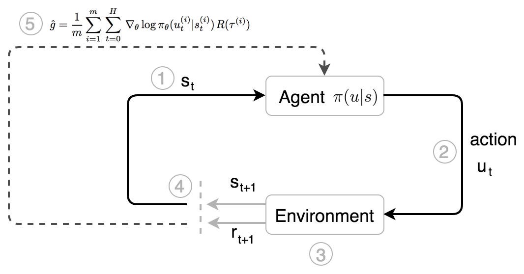
1. He observes the state of the environment (s).
2. He takes action (u) based on his instinct (a policy π) on the state s.
3. He moves and the opponents react. A new state is formed.
4. He takes further actions based on the observed state.
5. After a trajectory τ of motions, he adjusts his instinct based on the total rewards R(τ) received.

Curry visualizes the situation and instantly knows what to do. Years of training perfects the instinct to maximize the rewards. In RL, the instinct may be mathematically described as:

 

the probability of taking the action u given a state s. π is the policy in RL. For example, what is the chance of turning or stopping when you see a car in front:

 

Objective

How can we formulate our objective mathematically? The expected rewards equal the sum of the probability of a trajectory × corresponding rewards:

 

And our objective is to find a policy θ that create a trajectory τ

 

that maximizes the expected rewards.

 

Input features & rewards

 

s can be handcrafted features for the state (like the joint angles/velocity of a robotic arm) but in some problem domains, RL is mature enough to handle raw images directly. π can be a deterministic policy which output the exact action to be taken (move the joystick left or right). π can be a stochastic policy also which outputs the possibility of an action that it may take.

We record the reward r given at each time step. In a basketball game, all are 0 except the terminate state which equals 0, 1, 2 or 3.

 

Let’s introduce one more term H called the horizon. We can run the course of simulation indefinitely (h→∞) until it reaches the terminate state, or we set a limit to H steps.

Optimization

First, let’s identify a common and important trick in Deep Learning and RL. The partial derivative of a function f(x) (R.H.S.) is equal to f(x) times the partial derivative of the log(f(x)).

 

Replace f(x) with π.

 

Also, for a continuous space, expectation can be expressed as:

 

Now, let’s formalize our optimization problem mathematically. We want to model a policy that creates trajectories that maximize the total rewards.

 

However, to use gradient descent to optimize our problem, do we need to take the derivative of the reward function r which may not be differentiable or formalized?

Let’s rewrite our objective function J as:

 

The gradient (policy gradient) becomes:

 

Great news! The policy gradient can be represented as an expectation. It means we can use sampling to approximate it. Also, we sample the value of rbut not differentiate it. It makes sense because the rewards do not directly depend on how we parameterize the model. But the trajectories τ are. So what is the partial derivative of the log π(τ).

π(τ) is defined as:

 

Take the log:

 

The first and the last term does not depend on θ and can be removed.

 

So the policy gradient

 

becomes:

 

And we use this policy gradient to update the policy θ.

Intuition

 

How can we make sense of these equations? The underlined term is the maximum log likelihood. In deep learning, it measures the likelihood of the observed data. In our context, it measures how likely the trajectory is under the current policy. By multiplying it with the rewards, we want to increase the likelihood of a policy if the trajectory results in a high positive reward. On the contrary, we want to decrease the likelihood of a policy if it results in a high negative reward. In short, keep what is working and throw out what is not.

If going up the hill below means higher rewards, we will change the model parameters (policy) to increase the likelihood of trajectories that move higher.

 

Source

There is one thing significant about the policy gradient. The probability of a trajectory is defined as:

 

States in a trajectory are strongly related. In Deep Learning, a long sequence of multiplication with factors that are strongly correlated can trigger vanishing or exploding gradient easily. However, the policy gradient only sums up the gradient which breaks the curse of multiplying a long sequence of numbers.

 

The trick

 

creates a maximum log likelihood and the log breaks the curse of multiplying a long chain of policy.

Policy Gradient with Monte Carlo rollouts

Here is the REINFORCE algorithm which uses Monte Carlo rollout to compute the rewards. i.e. play out the whole episode to compute the total rewards.

 

Source

Policy gradient with automatic differentiation

The policy gradient can be computed easily with many Deep Learning software packages. For example, this is the partial code for TensorFlow:

 

Source

Yes, as often, coding looks simpler than the explanations.

Continuous control with Gaussian policies

How can we model a continuous control?

 

Let’s assume the values for actions are Gaussian distributed

 

and the policy is defined using a Gaussian distribution with means computed from a deep network:

 

With

 

We can compute the partial derivative of the log π as:

 

So we can backpropagate

 

through the policy network π to update the policy θ. The algorithm will look exactly the same as before. Just start with a slightly different way in calculating the log of the policy.

 

Source

Policy Gradients improvements

Policy Gradients suffer from high variance and low convergence.

Monte Carlo plays out the whole trajectory and records the exact rewards of a trajectory. However, the stochastic policy may take different actions in different episodes. One small turn can completely alter the result. So Monte Carlo has no bias but high variance. Variance hurts deep learning optimization. The variance provides conflicting descent direction for the model to learn. One sampled rewards may want to increase the log likelihood and another may want to decrease it. This hurts the convergence. To reduce the variance caused by actions, we want to reduce the variance for the sampled rewards.

 

Increasing the batch size in PG reduces variance.

However, increasing the batch size significantly reduces sample efficiency. So we cannot increase it too far, we need additional mechanisms to reduce the variance.

Baseline

 

We can always subtract a term to the optimization problem as long as the term is not related to θ. So instead of using the total reward, we subtract it with V(s).

 

We define the advantage function A and rewrite the policy gradient in terms of A.

 

In deep learning, we want input features to be zero-centered. Intuitively, RL is interested in knowing whether an action is performed better than the average. If rewards are always positive (R>0), PG always try to increase a trajectory probability even if it receives much smaller rewards than others. Consider two different situations:

• Situation 1: Trajectory A receives+10 rewards and Trajectory B receives -10 rewards.
• Situation 2: Trajectory A receives +10 rewards and Trajectory B receives +1 rewards.

In the first situation, PG will increase the probability of Trajectory A while decreasing B. In the second situation, it will increase both. As a human, we will likely decrease the likelihood of trajectory B in both situations.

By introducing a baseline, like V, we can recalibrate the rewards relative to the average action.

Vanilla Policy Gradient Algorithm

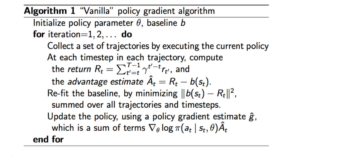
Here is the generic algorithm for the Policy Gradient Algorithm using a baseline b.

 

 

Source

Causality

Future actions should not change past decision. Present actions only impact the future. Therefore, we can change our objective function to reflect this also.

 

Reward discount

Reward discount reduces variance which reduces the impact of distant actions. Here, a different formula is used to compute the total rewards.

 

And the corresponding objective function becomes:

 

Part 2

This ends part 1 of the policy gradient methods. In the second part, we continue on the Temporal Difference, Hyperparameter tuning, and importance sampling. Temporal Difference will further reduce the variance and the importance sampling will lay down the theoretical foundation for more advanced policy gradient methods like TRPO and PPO.

RL — Policy Gradients Explained (Advanced topic)
In the first part of the Policy Gradients article, we cover the basic. In the second part, we continue on the Temporal…medium.com

Credit and references

UCL RL course

UC Berkeley RL course

UC Berkeley RL Bootcamp

A3C paper

GAE paper