TensorFlow使用记录 (三): Learning Rate Scheduling
file: tensorflow/python/training/learning_rate_decay.py
神经网络中通过超参数 learning rate,来控制每次参数更新的幅度。学习率太小会降低网络优化的速度,增加训练时间;学习率太大则可能导致可能导致参数在局部最优解两侧来回振荡,网络不能收敛。
tensorflow 定义了很多的 学习率衰减方式:
指数衰减 tf.train.exponential_decay()
指数衰减是比较常用的衰减方法,学习率是跟当前的训练轮次指数相关的。
tf.train.exponential_decay(

    learning_rate,     # 初始学习率

    global_step,       # 当前训练轮次

    decay_steps,       # 衰减周期

    decay_rate,        # 衰减率系数

    staircase=False,   # 定义是否是阶梯型衰减,还是连续衰减,默认是 False

    name=None

)

'''

decayed_learning_rate = learning_rate *

                      decay_rate ^ (global_step / decay_steps)

'''
示例代码:
import tensorflow as tf

import matplotlib.pyplot as plt

style1 = []

style2 = []

N = 200

with tf.Session() as sess:

  sess.run(tf.global_variables_initializer())

  for step in range(N):

    # 标准指数型衰减

    learing_rate1 = tf.train.exponential_decay(

      learning_rate=0.5, global_step=step, decay_steps=10, decay_rate=0.9, staircase=False)

    # 阶梯型衰减

    learing_rate2 = tf.train.exponential_decay(

      learning_rate=0.5, global_step=step, decay_steps=10, decay_rate=0.9, staircase=True)

    lr1 = sess.run([learing_rate1])

    lr2 = sess.run([learing_rate2])

    style1.append(lr1)

    style2.append(lr2)

step = range(N)

plt.plot(step, style1, 'g-', linewidth=2, label='exponential_decay')

plt.plot(step, style2, 'r--', linewidth=1, label='exponential_decay_staircase')

plt.title('exponential_decay')

plt.xlabel('step')

plt.ylabel('learing rate')

plt.legend(loc='upper right')

plt.tight_layout()

plt.show()

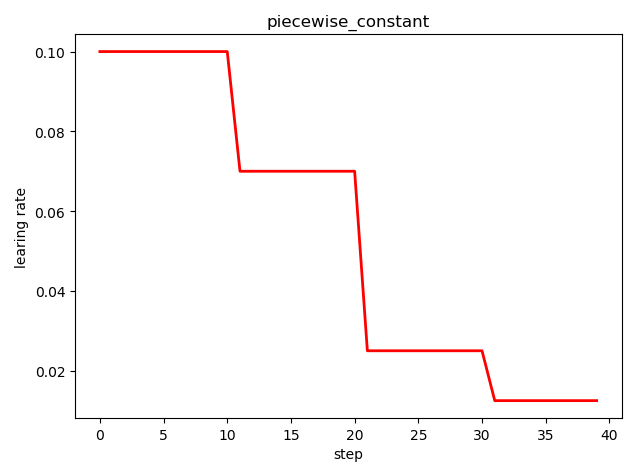
分段常数衰减 tf.train.piecewise_constant()
tf.train.piecewise_constant_decay(

    x,                # 当前训练轮次

    boundaries,       # 学习率应用区间

    values,           # 学习率常数列表

    name=None

)

'''

learning_rate value is `values[0]` when `x <= boundaries[0]`,

    `values[1]` when `x > boundaries[0]` and `x <= boundaries[1]`, ...,

    and values[-1] when `x > boundaries[-1]`.

'''
示例代码:
import tensorflow as tf

import matplotlib.pyplot as plt

boundaries = [10, 20, 30]

learing_rates = [0.1, 0.07, 0.025, 0.0125]

style = []

N = 40

with tf.Session() as sess:

  sess.run(tf.global_variables_initializer())

  for step in range(N):

    learing_rate = tf.train.piecewise_constant(step, boundaries=boundaries, values=learing_rates)

    lr = sess.run([learing_rate])

    style.append(lr)

step = range(N)

plt.plot(step, style, 'r-', linewidth=2)

plt.title('piecewise_constant')

plt.xlabel('step')

plt.ylabel('learing rate')

plt.tight_layout()

plt.show()
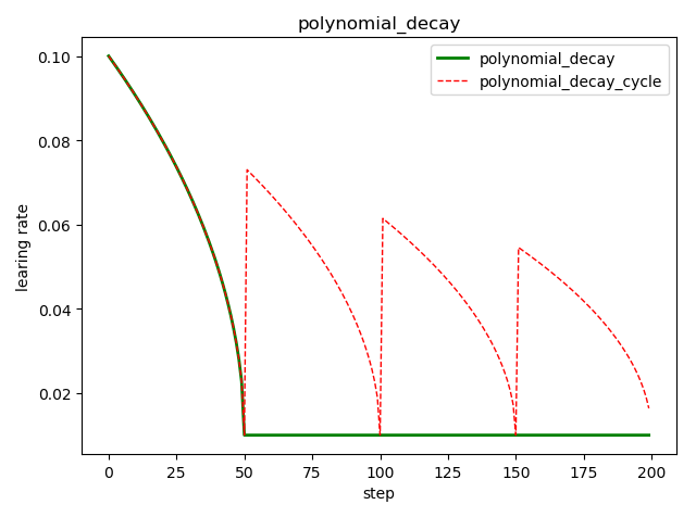
多项式衰减 tf.train.polynomial_decay()
tf.train.polynomial_decay(

    learning_rate,               # 初始学习率

    global_step,                 # 当前训练轮次

    decay_steps,                 # 大衰减周期

    end_learning_rate=0.0001,    # 最小的学习率

    power=1.0,                   # 多项式的幂

    cycle=False,                 # 学习率是否循环

    name=None)

'''

global_step = min(global_step, decay_steps)

decayed_learning_rate = (learning_rate - end_learning_rate) *

                        (1 - global_step / decay_steps) ^ (power) +

                         end_learning_rate

'''
示例代码:
import tensorflow as tf

import matplotlib.pyplot as plt

style1 = []

style2 = []

N = 200

with tf.Session() as sess:

  sess.run(tf.global_variables_initializer())

  for step in range(N):

    # cycle=False

    learing_rate1 = tf.train.polynomial_decay(

      learning_rate=0.1, global_step=step, decay_steps=50,

      end_learning_rate=0.01, power=0.5, cycle=False)

    # cycle=True

    learing_rate2 = tf.train.polynomial_decay(

      learning_rate=0.1, global_step=step, decay_steps=50,

      end_learning_rate=0.01, power=0.5, cycle=True)

    lr1 = sess.run([learing_rate1])

    lr2 = sess.run([learing_rate2])

    style1.append(lr1)

    style2.append(lr2)

steps = range(N)

plt.plot(steps, style1, 'g-', linewidth=2, label='polynomial_decay')

plt.plot(steps, style2, 'r--', linewidth=1, label='polynomial_decay_cycle')

plt.title('polynomial_decay')

plt.xlabel('step')

plt.ylabel('learing rate')

plt.legend(loc='upper right')

plt.tight_layout()

plt.show()
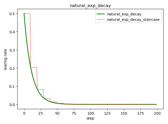
自然指数衰减 tf.train.natural_exp_decay()
tf.train.natural_exp_decay(

    learning_rate,        # 初始学习率

    global_step,          # 当前训练轮次

    decay_steps,          # 衰减周期

    decay_rate,           # 衰减率系数

    staircase=False,      # 定义是否是阶梯型衰减,还是连续衰减,默认是 False

    name=None

)

'''

decayed_learning_rate = learning_rate * exp(-decay_rate * global_step)

'''
示例代码:
import tensorflow as tf

import matplotlib.pyplot as plt

style1 = []

style2 = []

N = 200

with tf.Session() as sess:

  sess.run(tf.global_variables_initializer())

  for step in range(N):

    # 标准指数型衰减

    learing_rate1 = tf.train.natural_exp_decay(

      learning_rate=0.5, global_step=step, decay_steps=10, decay_rate=0.9, staircase=False)

    # 阶梯型衰减

    learing_rate2 = tf.train.natural_exp_decay(

      learning_rate=0.5, global_step=step, decay_steps=10, decay_rate=0.9, staircase=True)

    lr1 = sess.run([learing_rate1])

    lr2 = sess.run([learing_rate2])

    style1.append(lr1)

    style2.append(lr2)

step = range(N)

plt.plot(step, style1, 'g-', linewidth=2, label='natural_exp_decay')

plt.plot(step, style2, 'r--', linewidth=1, label='natural_exp_decay_staircase')

plt.title('natural_exp_decay')

plt.xlabel('step')

plt.ylabel('learing rate')

plt.legend(loc='upper right')

plt.tight_layout()

plt.show()
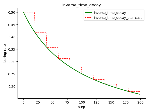
倒数衰减 tf.train.inverse_time_decay()
tf.train.inverse_time_decay(

    learning_rate,     # 初始学习率

    global_step,       # 当前训练轮次

    decay_steps,       # 衰减周期

    decay_rate,        # 衰减率系数

    staircase=False,   # 定义是否是阶梯型衰减,还是连续衰减,默认是 False

    name=None

)

'''

decayed_learning_rate = learning_rate / (1 + decay_rate * global_step / decay_step)

'''
示例代码:
import tensorflow as tf

import matplotlib.pyplot as plt

style1 = []

style2 = []

N = 200

with tf.Session() as sess:

  sess.run(tf.global_variables_initializer())

  for step in range(N):

    # 标准指数型衰减

    learing_rate1 = tf.train.inverse_time_decay(

      learning_rate=0.5, global_step=step, decay_steps=20, decay_rate=0.2, staircase=False)

    # 阶梯型衰减

    learing_rate2 = tf.train.inverse_time_decay(

      learning_rate=0.5, global_step=step, decay_steps=20, decay_rate=0.2, staircase=True)

    lr1 = sess.run([learing_rate1])

    lr2 = sess.run([learing_rate2])

    style1.append(lr1)

    style2.append(lr2)

step = range(N)

plt.plot(step, style1, 'g-', linewidth=2, label='inverse_time_decay')

plt.plot(step, style2, 'r--', linewidth=1, label='inverse_time_decay_staircase')

plt.title('inverse_time_decay')

plt.xlabel('step')

plt.ylabel('learing rate')

plt.legend(loc='upper right')

plt.tight_layout()

plt.show()
余弦衰减 tf.train.cosine_decay()
tf.train.cosine_decay(

    learning_rate,   # 初始学习率

    global_step,     # 当前训练轮次

    decay_steps,     # 衰减周期

    alpha=0.0,       # 最小的学习率

    name=None

)

'''

global_step = min(global_step, decay_steps)

cosine_decay = 0.5 * (1 + cos(pi * global_step / decay_steps))

decayed = (1 - alpha) * cosine_decay + alpha

decayed_learning_rate = learning_rate * decayed

'''
改进的余弦衰减方法还有:
线性余弦衰减,对应函数 tf.train.linear_cosine_decay()
噪声线性余弦衰减,对应函数 tf.train.noisy_linear_cosine_decay()
示例代码:
import tensorflow as tf

import matplotlib.pyplot as plt

style1 = []

style2 = []

style3 = []

N = 200

with tf.Session() as sess:

  sess.run(tf.global_variables_initializer())

  for step in range(N):

    # 余弦衰减

    learing_rate1 = tf.train.cosine_decay(

      learning_rate=0.1, global_step=step, decay_steps=50)

    # 线性余弦衰减

    learing_rate2 = tf.train.linear_cosine_decay(

      learning_rate=0.1, global_step=step, decay_steps=50)

    # 噪声线性余弦衰减

    learing_rate3 = tf.train.noisy_linear_cosine_decay(

      learning_rate=0.1, global_step=step, decay_steps=50,

      initial_variance=0.01, variance_decay=0.1, num_periods=0.2, alpha=0.5, beta=0.2)

    lr1 = sess.run([learing_rate1])

    lr2 = sess.run([learing_rate2])

    lr3 = sess.run([learing_rate3])

    style1.append(lr1)

    style2.append(lr2)

    style3.append(lr3)

step = range(N)

plt.plot(step, style1, 'g-', linewidth=2, label='cosine_decay')

plt.plot(step, style2, 'r--', linewidth=1, label='linear_cosine_decay')

plt.plot(step, style3, 'b--', linewidth=1, label='linear_cosine_decay')

plt.title('cosine_decay')

plt.xlabel('step')

plt.ylabel('learing rate')

plt.legend(loc='upper right')

plt.tight_layout()

plt.show()

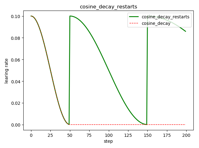
循环余弦衰减 tf.train.cosine_decay_restarts()
这是在 fast.ai 中强推的衰减方式
tf.train.cosine_decay_restarts(

    learning_rate,      # 初始学习率

    global_step,        # 当前训练轮次

    first_decay_steps,  # 首次衰减周期

    t_mul=2.0,          # 随后每次衰减周期倍数

    m_mul=1.0,          # 随后每次初始学习率倍数

    alpha=0.0,          # 最小的学习率=alpha*learning_rate

    name=None

)

'''

See [Loshchilov & Hutter, ICLR2016], SGDR: Stochastic Gradient Descent

with Warm Restarts. https://arxiv.org/abs/1608.03983

The learning rate multiplier first decays

from 1 to `alpha` for `first_decay_steps` steps. Then, a warm

restart is performed. Each new warm restart runs for `t_mul` times more steps

and with `m_mul` times smaller initial learning rate.

'''
示例代码:
import tensorflow as tf

import matplotlib.pyplot as plt

style1 = []

style2 = []

N = 200

with tf.Session() as sess:

  sess.run(tf.global_variables_initializer())

  for step in range(N):

    # 循环余弦衰减

    learing_rate1 = tf.train.cosine_decay_restarts(

      learning_rate=0.1, global_step=step, first_decay_steps=50,

      )

    # 余弦衰减

    learing_rate2 = tf.train.cosine_decay(

      learning_rate=0.1, global_step=step, decay_steps=50)

    lr1 = sess.run([learing_rate1])

    lr2 = sess.run([learing_rate2])

    style1.append(lr1)

    style2.append(lr2)

step = range(N)

plt.plot(step, style1, 'g-', linewidth=2, label='cosine_decay_restarts')

plt.plot(step, style2, 'r--', linewidth=1, label='cosine_decay')

plt.title('cosine_decay_restarts')

plt.xlabel('step')

plt.ylabel('learing rate')

plt.legend(loc='upper right')

plt.tight_layout()

plt.show()
调用例子
import tensorflow as tf

def Swish(features):

    return features*tf.nn.sigmoid(features)

# 1. create data

from tensorflow.examples.tutorials.mnist import input_data

mnist = input_data.read_data_sets('../MNIST_data', one_hot=True)

X = tf.placeholder(tf.float32, shape=(None, 784), name='X')

y = tf.placeholder(tf.int32, shape=(None), name='y')

is_training = tf.placeholder(tf.bool, None, name='is_training')

# 2. define network

he_init = tf.contrib.layers.variance_scaling_initializer()

with tf.name_scope('dnn'):

    hidden1 = tf.layers.dense(X, 300, kernel_initializer=he_init, name='hidden1')

    hidden1 = tf.layers.batch_normalization(hidden1, momentum=0.9)

    hidden1 = tf.nn.relu(hidden1)

    hidden2 = tf.layers.dense(hidden1, 100, kernel_initializer=he_init, name='hidden2')

    hidden2 = tf.layers.batch_normalization(hidden2, training=is_training, momentum=0.9)

    hidden2 = tf.nn.relu(hidden2)

    logits = tf.layers.dense(hidden2, 10, kernel_initializer=he_init, name='output')

    # prob = tf.layers.dense(hidden2, 10, tf.nn.softmax, name='prob')

# 3. define loss

with tf.name_scope('loss'):

    # tf.losses.sparse_softmax_cross_entropy() label is not one_hot and dtype is int*

    # xentropy = tf.losses.sparse_softmax_cross_entropy(labels=tf.argmax(y, axis=1), logits=logits)

    # tf.nn.sparse_softmax_cross_entropy_with_logits() label is not one_hot and dtype is int*

    # xentropy = tf.nn.sparse_softmax_cross_entropy_with_logits(labels=tf.argmax(y, axis=1), logits=logits)

    # loss = tf.reduce_mean(xentropy)

    loss = tf.losses.softmax_cross_entropy(onehot_labels=y, logits=logits) # label is one_hot

# 4. define optimizer

learning_rate_init = 0.01

global_step = tf.Variable(0, trainable=False)

with tf.name_scope('train'):

    learning_rate = tf.train.polynomial_decay(  # 多项式衰减

        learning_rate=learning_rate_init,  # 初始学习率

        global_step=global_step,  # 当前迭代次数

        decay_steps=22000,  # 在迭代到该次数实际,学习率衰减为 learning_rate * dacay_rate

        end_learning_rate=learning_rate_init / 10,  # 最小的学习率

        power=0.9,

        cycle=False

    )

    update_ops = tf.get_collection(tf.GraphKeys.UPDATE_OPS)  # for batch normalization

    with tf.control_dependencies(update_ops):

        optimizer_op = tf.train.GradientDescentOptimizer(

            learning_rate=learning_rate).minimize(

            loss=loss,

            var_list=tf.trainable_variables(),

            global_step=global_step # 不指定的话学习率不更新

        )

        # ================= clip gradient

        # threshold = 1.0

        # optimizer = tf.train.GradientDescentOptimizer(learning_rate)

        # grads_and_vars = optimizer.compute_gradients(loss)

        # capped_gvs = [(tf.clip_by_value(grad, -threshold, threshold), var)

        #               for grad, var in grads_and_vars]

        # optimizer_op = optimizer.apply_gradients(capped_gvs)

        # =================

with tf.name_scope('eval'):

    correct = tf.nn.in_top_k(logits, tf.argmax(y, axis=1), 1) # 目标是否在前K个预测中, label's dtype is int*

    accuracy = tf.reduce_mean(tf.cast(correct, tf.float32))

# 5. initialize

init_op = tf.group(tf.global_variables_initializer(), tf.local_variables_initializer())

saver = tf.train.Saver()

# =================

print([v.name for v in tf.trainable_variables()])

print([v.name for v in tf.global_variables()])

# =================

# 6. train & test

n_epochs = 20

n_batches = 50

batch_size = 50

with tf.Session() as sess:

    sess.run(init_op)

    # saver.restore(sess, './my_model_final.ckpt')

    for epoch in range(n_epochs):

        for iteration in range(mnist.train.num_examples // batch_size):

            X_batch, y_batch = mnist.train.next_batch(batch_size)

            sess.run([optimizer_op, learning_rate], feed_dict={X: X_batch, y: y_batch, is_training:True})

            # ================= check gradient

            # for grad, var in grads_and_vars:

            #     grad = grad.eval(feed_dict={X: X_batch, y: y_batch, is_training:True})

            #     var = var.eval()

            # =================

        learning_rate_cur = learning_rate.eval()

        acc_train = accuracy.eval(feed_dict={X: X_batch, y: y_batch, is_training:False}) # 最后一个 batch 的 accuracy

        acc_test = accuracy.eval(feed_dict={X: mnist.test.images, y: mnist.test.labels, is_training:False})

        loss_test = loss.eval(feed_dict={X: mnist.test.images, y: mnist.test.labels, is_training:False})

        print(epoch, "Current learning rate:", learning_rate_cur, "Train accuracy:", acc_train, "Test accuracy:", acc_test, "Test loss:", loss_test)

    save_path = saver.save(sess, "./my_model_final.ckpt")

with tf.Session() as sess:

    sess.run(init_op)

    saver.restore(sess, "./my_model_final.ckpt")

    acc_test = accuracy.eval(feed_dict={X: mnist.test.images, y: mnist.test.labels, is_training:False})

    loss_test = loss.eval(feed_dict={X: mnist.test.images, y: mnist.test.labels, is_training:False})

    print("Test accuracy:", acc_test, ", Test loss:", loss_test)
Since AdaGrad, RMSProp, and Adam optimization automatically reduce the learning rate during training, it is not necessary to add an extra learning schedule. For other optimization algorithms, using exponential decay or performance scheduling can considerably speed up convergence.
TensorFlow使用记录 (三): Learning Rate Scheduling的更多相关文章
- 5、Tensorflow基础(三)神经元函数及优化方法
1.激活函数 激活函数(activation function)运行时激活神经网络中某一部分神经元,将激活信息向后传入下一层的神经网络.神经网络之所以能解决非线性问题(如语音.图像识别),本质上就是激 ...
- Deep Learning 32: 自己写的keras的一个callbacks函数,解决keras中不能在每个epoch实时显示学习速率learning rate的问题
一.问题: keras中不能在每个epoch实时显示学习速率learning rate,从而方便调试,实际上也是为了调试解决这个问题:Deep Learning 31: 不同版本的keras,对同样的 ...
- TensorFlow使用记录 (九): 模型保存与恢复
模型文件 tensorflow 训练保存的模型注意包含两个部分:网络结构和参数值. .meta .meta 文件以 “protocol buffer”格式保存了整个模型的结构图,模型上定义的操作等信息 ...
- TensorFlow使用记录 (六): 优化器
0. tf.train.Optimizer tensorflow 里提供了丰富的优化器,这些优化器都继承与 Optimizer 这个类.class Optimizer 有一些方法,这里简单介绍下: 0 ...
- tensorflow笔记(三)之 tensorboard的使用
tensorflow笔记(三)之 tensorboard的使用 版权声明:本文为博主原创文章,转载请指明转载地址 http://www.cnblogs.com/fydeblog/p/7429344.h ...
- mxnet设置动态学习率(learning rate)
https://blog.csdn.net/xiaotao_1/article/details/78874336 如果learning rate很大,算法会在局部最优点附近来回跳动,不会收敛: 如果l ...
- TensorFlow使用记录 (八): 梯度修剪 和 Max-Norm Regularization
梯度修剪 梯度修剪主要避免训练梯度爆炸的问题,一般来说使用了 Batch Normalization 就不必要使用梯度修剪了,但还是有必要理解下实现的 In TensorFlow, the optim ...
- TensorFlow实战第三课(可视化、加速神经网络训练)
matplotlib可视化 构件图形 用散点图描述真实数据之间的关系(plt.ion()用于连续显示) # plot the real data fig = plt.figure() ax = fig ...
- Dynamic learning rate in training - 培训中的动态学习率
I'm using keras 2.1.* and want to change the learning rate during training. I know about the schedul ...
随机推荐
- Oracle-DDL 1- 表管理
DDL-数据定义语句: 一.表管理 1.create 创建表-- 必须有创建表的权限和表空间-- 表名必须以字母开头,可以包含数字和符号,不能是系统关键字 /*create table 表名(列名1 ...
- Oracle表的Rowid字段
Rowid 字段类型: Rowid 是一行数据的一个唯一标识. ROWID 是数据的详细地址,通过 rowid,oracle 可以快速的定位某行具体的数据的位置. ROWID 可以分为物理 rowid ...
- 为什么说Python采用的是基于值的内存管理模式?
Python中的变量并不直接存储值,而是存储了值的内存地址或者引用,假如为不同变量赋值为相同值,这个值在内存中只有一份,多个变量指向同一块内存地址.
- Bash Plays with Functions CodeForces - 757E (积性函数dp)
大意: 定义函数$f_r(n)$, $f_0(n)$为pq=n且gcd(p,q)=1的有序对(p,q)个数. $r \ge 1$时, $f_r(n)=\sum\limits_{uv=n}\frac{f ...
- python:enumerate 函数
说明 enumerate()是python的内置函数: 对于一个可迭代的(iterable)/可遍历的对象(如列表.字符串),enumerate将其组成一个索引序列,利用它可以同时获得索引和值 多用于 ...
- scrapy-redis 实现分布式爬虫
分布式爬虫 一 介绍 原来scrapy的Scheduler维护的是本机的任务队列(存放Request对象及其回调函数等信息)+本机的去重队列(存放访问过的url地址) 所以实现分布式爬取的关键就是,找 ...
- 使用nodejs开发一个markdown文档管理小系统(一)Using Nodejs to quickly develop a markdown management system
好多年没碰过前端jquery了,用一两天时间重温一下,刚好写个小工具, 不递归取文件夹和文件,只写一层,保持足够简单,验证和参数判断暂不写,毕竟只写了几个小时而已,功能算完备了,添加一个简单的管理员权 ...
- C++的一些黑暗料理
本文中的“黑暗料理”仅限本人在学习C++的过程中感觉易忘.有趣.不为大多数人所知的一些特性. 1. C++中int型数据在VC++环境下最小值为什么是 -32678,而不是-32677,其中涉及到原码 ...
- STL源码阅读-traits与迭代器
迭代器模式 提供一种方法,使之能够依序访问容器的各个元素,而又无需暴露容器的内部表述方式 STL设计的中心思想在于将数据容器和算法分离开,容器和算法分开设计,迭代器则是两者之间的胶着剂,一般迭代器的设 ...
- string::find_first_not_of
string (1) size_t find_first_not_of (const string& str, size_t pos = 0) const noexcept; c-string ...