fast planner总结

一、前端 kinodynamic A*算法动力学路径搜索

1.1 路径搜索的主要函数为kinodynamicAstar类的search函数

int KinodynamicAstar::search(Eigen::Vector3d start_pt, Eigen::Vector3d start_v, Eigen::Vector3d start_a,
                             Eigen::Vector3d end_pt, Eigen::Vector3d end_v, bool init, bool dynamic, double time_start)
{
//初始化参数
  start_vel_ = start_v;
  start_acc_ = start_a;

  PathNodePtr cur_node = path_node_pool_[0];
  cur_node->parent = NULL;
  cur_node->state.head(3) = start_pt;
  cur_node->state.tail(3) = start_v;
  cur_node->index = posToIndex(start_pt);
  cur_node->g_score = 0.0;

  Eigen::VectorXd end_state(6);
  Eigen::Vector3i end_index;
  double time_to_goal;

  end_state.head(3) = end_pt;
  end_state.tail(3) = end_v;
  end_index = posToIndex(end_pt);
  cur_node->f_score = lambda_heu_ * estimateHeuristic(cur_node->state, end_state, time_to_goal);
  cur_node->node_state = IN_OPEN_SET;
  open_set_.push(cur_node);
  use_node_num_ += 1;

  if (dynamic)
  {
    time_origin_ = time_start;
    cur_node->time = time_start;
    cur_node->time_idx = timeToIndex(time_start);
    expanded_nodes_.insert(cur_node->index, cur_node->time_idx, cur_node);
    // cout << "time start: " << time_start << endl;
  }
  else
    expanded_nodes_.insert(cur_node->index, cur_node);

  PathNodePtr neighbor = NULL;
  PathNodePtr terminate_node = NULL;
  bool init_search = init;
  const int tolerance = ceil(1 / resolution_);

  while (!open_set_.empty())
  {
    cur_node = open_set_.top();

    // Terminate?
    bool reach_horizon = (cur_node->state.head(3) - start_pt).norm() >= horizon_;
    bool near_end = abs(cur_node->index(0) - end_index(0)) <= tolerance &&
                    abs(cur_node->index(1) - end_index(1)) <= tolerance &&
                    abs(cur_node->index(2) - end_index(2)) <= tolerance;

//当前节点超出horizon或接近目标点，计算一条直达的曲线，并检查曲线是否存在。
//主要为了解决稀疏采样，最终不能精准的到达目标点的问题
    if (reach_horizon || near_end)
    {
      terminate_node = cur_node;
      retrievePath(terminate_node);
      if (near_end)
      {
        // Check whether shot traj exist
        estimateHeuristic(cur_node->state, end_state, time_to_goal);
        computeShotTraj(cur_node->state, end_state, time_to_goal);
        if (init_search)
          ROS_ERROR("Shot in first search loop!");
      }
    }
    if (reach_horizon)
    {
      if (is_shot_succ_)
      {
        std::cout << "reach end" << std::endl;
        return REACH_END;
      }
      else
      {
        std::cout << "reach horizon" << std::endl;
        return REACH_HORIZON;
      }
    }

    if (near_end)
    {
      if (is_shot_succ_)
      {
        std::cout << "reach end" << std::endl;
        return REACH_END;
      }
      else if (cur_node->parent != NULL)
      {
        std::cout << "near end" << std::endl;
        return NEAR_END;
      }
      else
      {
        std::cout << "no path" << std::endl;
        return NO_PATH;
      }
    }

    //开始节点扩展
    open_set_.pop();
    cur_node->node_state = IN_CLOSE_SET;
    iter_num_ += 1;

    double res = 1 / 2.0, time_res = 1 / 1.0, time_res_init = 1 / 20.0;
    Eigen::Matrix<double, 6, 1> cur_state = cur_node->state;
    Eigen::Matrix<double, 6, 1> pro_state;
    vector<PathNodePtr> tmp_expand_nodes;
    Eigen::Vector3d um;
    double pro_t;
    vector<Eigen::Vector3d> inputs;
    vector<double> durations;
    //获取采样输入
    if (init_search)
    {
      inputs.push_back(start_acc_);
      for (double tau = time_res_init * init_max_tau_; tau <= init_max_tau_ + 1e-3;
           tau += time_res_init * init_max_tau_)
        durations.push_back(tau);
      init_search = false;
    }
    else
    {
      for (double ax = -max_acc_; ax <= max_acc_ + 1e-3; ax += max_acc_ * res)
        for (double ay = -max_acc_; ay <= max_acc_ + 1e-3; ay += max_acc_ * res)
          for (double az = -max_acc_; az <= max_acc_ + 1e-3; az += max_acc_ * res)
          {
            um << ax, ay, az;
            inputs.push_back(um);  //输入也储存下，方便后面采样用
          }
      for (double tau = time_res * max_tau_; tau <= max_tau_; tau += time_res * max_tau_)
        durations.push_back(tau);  //输入持续时间
    }

    // cout << "cur state:" << cur_state.head(3).transpose() << endl;
    for (int i = 0; i < inputs.size(); ++i)
      for (int j = 0; j < durations.size(); ++j)
      {
        um = inputs[i];
        double tau = durations[j];
        stateTransit(cur_state, pro_state, um, tau);   //前向积分成路径
        pro_t = cur_node->time + tau;

        Eigen::Vector3d pro_pos = pro_state.head(3);

        // Check if in close set
        Eigen::Vector3i pro_id = posToIndex(pro_pos);
        int pro_t_id = timeToIndex(pro_t);
        PathNodePtr pro_node = dynamic ? expanded_nodes_.find(pro_id, pro_t_id) : expanded_nodes_.find(pro_id);
        if (pro_node != NULL && pro_node->node_state == IN_CLOSE_SET)
        {
          if (init_search)
            std::cout << "close" << std::endl;
          continue;
        }

        // Check maximal velocity
        Eigen::Vector3d pro_v = pro_state.tail(3);
        if (fabs(pro_v(0)) > max_vel_ || fabs(pro_v(1)) > max_vel_ || fabs(pro_v(2)) > max_vel_)
        {
          if (init_search)
            std::cout << "vel" << std::endl;
          continue;
        }

        // Check not in the same voxel
        Eigen::Vector3i diff = pro_id - cur_node->index;
        int diff_time = pro_t_id - cur_node->time_idx;
        if (diff.norm() == 0 && ((!dynamic) || diff_time == 0))
        {
          if (init_search)
            std::cout << "same" << std::endl;
          continue;
        }

        // Check safety
        Eigen::Vector3d pos;
        Eigen::Matrix<double, 6, 1> xt;
        bool is_occ = false;
        for (int k = 1; k <= check_num_; ++k)
        {
          double dt = tau * double(k) / double(check_num_);
          stateTransit(cur_state, xt, um, dt);
          pos = xt.head(3);
          if (edt_environment_->sdf_map_->getInflateOccupancy(pos) == 1 )
          {
            is_occ = true;
            break;
          }
        }
        if (is_occ)
        {
          if (init_search)
            std::cout << "safe" << std::endl;
          continue;
        }
    //计算代价
        double time_to_goal, tmp_g_score, tmp_f_score;
        tmp_g_score = (um.squaredNorm() + w_time_) * tau + cur_node->g_score;
        tmp_f_score = tmp_g_score + lambda_heu_ * estimateHeuristic(pro_state, end_state, time_to_goal);
    //节点裁剪
/*********
首先判断当前临时扩展节点与current node的其他临时扩展节点是否在同一个voxel中，如果是的话，
就要进行剪枝。要判断当前临时扩展节点的fscore是否比同一个voxel的对比fscore小，如果是的话，
则更新这一Voxel节点为当前临时扩展节点。

如果不剪枝的话，则首先判断当前临时扩展节点pro_node是否出现在open集中，如果是不是的话，
则可以直接将pro_node加入open集中。如果存在于open集但还未扩展的话，
则比较当前临时扩展节点与对应VOXEL节点的fscore,若更小，则更新voxel中的节点。

需要进行说明的是，在Fast planner的实现中，open集是通过两个数据结构实现的，
一个队列用来存储，弹出open集中的节点。
另一个哈希表NodeHashtable 用来查询节点是否已经存在于open集中。
而判断一个节点是否存在于close set中，则是通过Nodehashtable 与nodestate来决定的，如果nodeState 是 InCloseSet, 且存在于NodeHashtable,
则说明该节点已经被扩展过了，存在于close set中。
*****************/
        // Compare nodes expanded from the same parent
        bool prune = false;
        for (int j = 0; j < tmp_expand_nodes.size(); ++j)
        {
          PathNodePtr expand_node = tmp_expand_nodes[j];

          if ((pro_id - expand_node->index).norm() == 0 && ((!dynamic) || pro_t_id == expand_node->time_idx))
          {
            prune = true;
            if (tmp_f_score < expand_node->f_score)
            {
              expand_node->f_score = tmp_f_score;
              expand_node->g_score = tmp_g_score;
              expand_node->state = pro_state;
              expand_node->input = um;
              expand_node->duration = tau;
              if (dynamic)
                expand_node->time = cur_node->time + tau;
            }
            break;
          }
        }

        // This node end up in a voxel different from others
        if (!prune)
        {
          if (pro_node == NULL)
          {
            pro_node = path_node_pool_[use_node_num_];
            pro_node->index = pro_id;
            pro_node->state = pro_state;
            pro_node->f_score = tmp_f_score;
            pro_node->g_score = tmp_g_score;
            pro_node->input = um;
            pro_node->duration = tau;
            pro_node->parent = cur_node;
            pro_node->node_state = IN_OPEN_SET;
            if (dynamic)
            {
              pro_node->time = cur_node->time + tau;
              pro_node->time_idx = timeToIndex(pro_node->time);
            }
            open_set_.push(pro_node);

            if (dynamic)
              expanded_nodes_.insert(pro_id, pro_node->time, pro_node);
            else
              expanded_nodes_.insert(pro_id, pro_node);

            tmp_expand_nodes.push_back(pro_node);

            use_node_num_ += 1;
            if (use_node_num_ == allocate_num_)
            {
              cout << "run out of memory." << endl;
              return NO_PATH;
            }
          }
          else if (pro_node->node_state == IN_OPEN_SET)
          {
            if (tmp_g_score < pro_node->g_score)
            {
              // pro_node->index = pro_id;
              pro_node->state = pro_state;
              pro_node->f_score = tmp_f_score;
              pro_node->g_score = tmp_g_score;
              pro_node->input = um;
              pro_node->duration = tau;
              pro_node->parent = cur_node;
              if (dynamic)
                pro_node->time = cur_node->time + tau;
            }
          }
          else
          {
            cout << "error type in searching: " << pro_node->node_state << endl;
          }
        }
      }
    // init_search = false;
  }

  cout << "open set empty, no path!" << endl;
  cout << "use node num: " << use_node_num_ << endl;
  cout << "iter num: " << iter_num_ << endl;
  return NO_PATH;
}

1.2 启发式函数设置

主要是利用庞特里亚金原理解决两点边界问题，得到最优解后，同时得到代价。



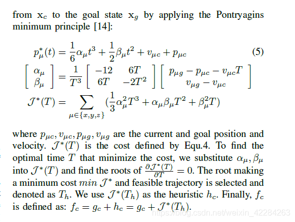
首先通过设置启发函数对时间求导等于0，得到启发函数关于时间T的四次方程，再通过求解该四次方程，得到一系列实根，通过比较这些实根所对应的cost大小，得到最优时间。这里需要注意，关于时间的一元四次方程是通过费拉里方法求解的，需要嵌套一个元三次方程进行求解，也就是代码中应的cubic（）函数。

double KinodynamicAstar::estimateHeuristic(Eigen::VectorXd x1, Eigen::VectorXd x2, double& optimal_time)
{
  const Vector3d dp = x2.head(3) - x1.head(3);
  const Vector3d v0 = x1.segment(3, 3);
  const Vector3d v1 = x2.segment(3, 3);

  double c1 = -36 * dp.dot(dp);
  double c2 = 24 * (v0 + v1).dot(dp);
  double c3 = -4 * (v0.dot(v0) + v0.dot(v1) + v1.dot(v1));
  double c4 = 0;
  double c5 = w_time_;

  std::vector<double> ts = quartic(c5, c4, c3, c2, c1);

  double v_max = max_vel_ * 0.5;
  double t_bar = (x1.head(3) - x2.head(3)).lpNorm<Infinity>() / v_max;
  ts.push_back(t_bar);

  double cost = 100000000;
  double t_d = t_bar;

  for (auto t : ts)
  {
    if (t < t_bar)
      continue;
    double c = -c1 / (3 * t * t * t) - c2 / (2 * t * t) - c3 / t + w_time_ * t;
    if (c < cost)
    {
      cost = c;
      t_d = t;
    }
  }

  optimal_time = t_d;

  return 1.0 * (1 + tie_breaker_) * cost;
}

公式推导参考：https://blog.csdn.net/qq_16775293/article/details/124845417

1.3 这里我们遇到了第二个重要的函数ComputeShotTraj. 即利用庞特里亚金原理解一个两点边值问题。因为最优控制时间已经在estimateHeuristic中计算过了，所以这里只要引入该时间进行多项式计算即可。这部分的目的是为了验证该轨迹是安全的，即不发生碰撞，速度、加速度不超限。

bool KinodynamicAstar::computeShotTraj(Eigen::VectorXd state1, Eigen::VectorXd state2, double time_to_goal)
{
  /* ---------- get coefficient ---------- */
  const Vector3d p0 = state1.head(3);
  const Vector3d dp = state2.head(3) - p0;
  const Vector3d v0 = state1.segment(3, 3);
  const Vector3d v1 = state2.segment(3, 3);
  const Vector3d dv = v1 - v0;
  double t_d = time_to_goal;
  MatrixXd coef(3, 4);
  end_vel_ = v1;

  Vector3d a = 1.0 / 6.0 * (-12.0 / (t_d * t_d * t_d) * (dp - v0 * t_d) + 6 / (t_d * t_d) * dv);
  Vector3d b = 0.5 * (6.0 / (t_d * t_d) * (dp - v0 * t_d) - 2 / t_d * dv);
  Vector3d c = v0;
  Vector3d d = p0;

  // 1/6 * alpha * t^3 + 1/2 * beta * t^2 + v0
  // a*t^3 + b*t^2 + v0*t + p0
  coef.col(3) = a, coef.col(2) = b, coef.col(1) = c, coef.col(0) = d;

  Vector3d coord, vel, acc;
  VectorXd poly1d, t, polyv, polya;
  Vector3i index;

  Eigen::MatrixXd Tm(4, 4);
  Tm << 0, 1, 0, 0, 0, 0, 2, 0, 0, 0, 0, 3, 0, 0, 0, 0;

  /* ---------- forward checking of trajectory ---------- */
  double t_delta = t_d / 10;
  for (double time = t_delta; time <= t_d; time += t_delta)
  {
    t = VectorXd::Zero(4);
    for (int j = 0; j < 4; j++)
      t(j) = pow(time, j);

    for (int dim = 0; dim < 3; dim++)
    {
      poly1d = coef.row(dim);
      coord(dim) = poly1d.dot(t);
      vel(dim) = (Tm * poly1d).dot(t);
      acc(dim) = (Tm * Tm * poly1d).dot(t);

      if (fabs(vel(dim)) > max_vel_ || fabs(acc(dim)) > max_acc_)
      {
        // cout << "vel:" << vel(dim) << ", acc:" << acc(dim) << endl;
        // return false;
      }
    }

    if (coord(0) < origin_(0) || coord(0) >= map_size_3d_(0) || coord(1) < origin_(1) || coord(1) >= map_size_3d_(1) ||
        coord(2) < origin_(2) || coord(2) >= map_size_3d_(2))
    {
      return false;
    }

    // if (edt_environment_->evaluateCoarseEDT(coord, -1.0) <= margin_) {
    //   return false;
    // }
    if (edt_environment_->sdf_map_->getInflateOccupancy(coord) == 1)
    {
      return false;
    }
  }
  coef_shot_ = coef;
  t_shot_ = t_d;
  is_shot_succ_ = true;
  return true;
}

二、后端优化

2.1 离散采样，获取一些轨迹点和速度、加速度。

void KinodynamicAstar::getSamples(double& ts, vector<Eigen::Vector3d>& point_set,
                                  vector<Eigen::Vector3d>& start_end_derivatives)
{
  /* ---------- path duration ---------- */
  double T_sum = 0.0;
  if (is_shot_succ_)
    T_sum += t_shot_;
  PathNodePtr node = path_nodes_.back();
  while (node->parent != NULL)
  {
    T_sum += node->duration;
    node = node->parent;
  }
  // cout << "duration:" << T_sum << endl;

  // Calculate boundary vel and acc
  Eigen::Vector3d end_vel, end_acc;
  double t;
  if (is_shot_succ_)
  {
    t = t_shot_;
    end_vel = end_vel_;
    for (int dim = 0; dim < 3; ++dim)
    {
      Vector4d coe = coef_shot_.row(dim);
      end_acc(dim) = 2 * coe(2) + 6 * coe(3) * t_shot_;
    }
  }
  else
  {
    t = path_nodes_.back()->duration;
    end_vel = node->state.tail(3);
    end_acc = path_nodes_.back()->input;
  }

  // Get point samples
  int seg_num = floor(T_sum / ts);
  seg_num = max(8, seg_num);
  ts = T_sum / double(seg_num);
  bool sample_shot_traj = is_shot_succ_;
  node = path_nodes_.back();

  for (double ti = T_sum; ti > -1e-5; ti -= ts)
  {
    if (sample_shot_traj)
    {
      // samples on shot traj
      Vector3d coord;
      Vector4d poly1d, time;

      for (int j = 0; j < 4; j++)
        time(j) = pow(t, j);

      for (int dim = 0; dim < 3; dim++)
      {
        poly1d = coef_shot_.row(dim);
        coord(dim) = poly1d.dot(time);
      }

      point_set.push_back(coord);
      t -= ts;

      /* end of segment */
      if (t < -1e-5)
      {
        sample_shot_traj = false;
        if (node->parent != NULL)
          t += node->duration;
      }
    }
    else
    {
      // samples on searched traj
      Eigen::Matrix<double, 6, 1> x0 = node->parent->state;
      Eigen::Matrix<double, 6, 1> xt;
      Vector3d ut = node->input;

      stateTransit(x0, xt, ut, t);

      point_set.push_back(xt.head(3));
      t -= ts;

      // cout << "t: " << t << ", t acc: " << T_accumulate << endl;
      if (t < -1e-5 && node->parent->parent != NULL)
      {
        node = node->parent;
        t += node->duration;
      }
    }
  }
  reverse(point_set.begin(), point_set.end());

  // calculate start acc
  Eigen::Vector3d start_acc;
  if (path_nodes_.back()->parent == NULL)
  {
    // no searched traj, calculate by shot traj
    start_acc = 2 * coef_shot_.col(2);
  }
  else
  {
    // input of searched traj
    start_acc = node->input;
  }

  start_end_derivatives.push_back(start_vel_);
  start_end_derivatives.push_back(end_vel);
  start_end_derivatives.push_back(start_acc);
  start_end_derivatives.push_back(end_acc);
}

2.2 前端离散点拟合成B样条曲线

每获得一个轨迹点就认为是一段？就有多少个控制点？这样控制点有点多啊

void NonUniformBspline::parameterizeToBspline(const double& ts, const vector<Eigen::Vector3d>& point_set,
                                              const vector<Eigen::Vector3d>& start_end_derivative,
                                              Eigen::MatrixXd&               ctrl_pts) {
  if (ts <= 0) {
    cout << "[B-spline]:time step error." << endl;
    return;
  }

  if (point_set.size() < 2) {
    cout << "[B-spline]:point set have only " << point_set.size() << " points." << endl;
    return;
  }

  if (start_end_derivative.size() != 4) {
    cout << "[B-spline]:derivatives error." << endl;
  }

  int K = point_set.size();

  // write A
  Eigen::Vector3d prow(3), vrow(3), arow(3);
  prow << 1, 4, 1;
  vrow << -1, 0, 1;
  arow << 1, -2, 1;

  Eigen::MatrixXd A = Eigen::MatrixXd::Zero(K + 4, K + 2);

  for (int i = 0; i < K; ++i) A.block(i, i, 1, 3) = (1 / 6.0) * prow.transpose();

  A.block(K, 0, 1, 3)         = (1 / 2.0 / ts) * vrow.transpose();
  A.block(K + 1, K - 1, 1, 3) = (1 / 2.0 / ts) * vrow.transpose();

  A.block(K + 2, 0, 1, 3)     = (1 / ts / ts) * arow.transpose();
  A.block(K + 3, K - 1, 1, 3) = (1 / ts / ts) * arow.transpose();
  // cout << "A:\n" << A << endl;

  // A.block(0, 0, K, K + 2) = (1 / 6.0) * A.block(0, 0, K, K + 2);
  // A.block(K, 0, 2, K + 2) = (1 / 2.0 / ts) * A.block(K, 0, 2, K + 2);
  // A.row(K + 4) = (1 / ts / ts) * A.row(K + 4);
  // A.row(K + 5) = (1 / ts / ts) * A.row(K + 5);

  // write b
  Eigen::VectorXd bx(K + 4), by(K + 4), bz(K + 4);
  for (int i = 0; i < K; ++i) {
    bx(i) = point_set[i](0);
    by(i) = point_set[i](1);
    bz(i) = point_set[i](2);
  }

  for (int i = 0; i < 4; ++i) {
    bx(K + i) = start_end_derivative[i](0);
    by(K + i) = start_end_derivative[i](1);
    bz(K + i) = start_end_derivative[i](2);
  }

  // solve Ax = b
  Eigen::VectorXd px = A.colPivHouseholderQr().solve(bx);
  Eigen::VectorXd py = A.colPivHouseholderQr().solve(by);
  Eigen::VectorXd pz = A.colPivHouseholderQr().solve(bz);

  // convert to control pts
  ctrl_pts.resize(K + 2, 3);
  ctrl_pts.col(0) = px;
  ctrl_pts.col(1) = py;
  ctrl_pts.col(2) = pz;

  // cout << "[B-spline]: parameterization ok." << endl;
}

虽然在计算B样条曲线上某一点的值时论文用的是DeBoor公式，但是在使用均匀B样条对前端路径进行拟合时用的是B样条的矩阵表达方法，具体参见论文：K. Qin, “General matrix representations for b-splines,” The Visual Computer, vol. 16, no. 3, pp. 177–186, 2000.

2.3 B样条优化

Eigen::MatrixXd BsplineOptimizer::BsplineOptimizeTraj(const Eigen::MatrixXd& points, const double& ts,
                                                      const int& cost_function, int max_num_id,
                                                      int max_time_id) {
  setControlPoints(points);
  setBsplineInterval(ts);
  setCostFunction(cost_function);
  setTerminateCond(max_num_id, max_time_id);

  optimize();
  return this->control_points_;
}

void BsplineOptimizer::optimize() {
  /* initialize solver */
  iter_num_        = 0;
  min_cost_        = std::numeric_limits<double>::max();
  const int pt_num = control_points_.rows();
  g_q_.resize(pt_num);
  g_smoothness_.resize(pt_num);
  g_distance_.resize(pt_num);
  g_feasibility_.resize(pt_num);
  g_endpoint_.resize(pt_num);
  g_waypoints_.resize(pt_num);
  g_guide_.resize(pt_num);

  if (cost_function_ & ENDPOINT) {
    variable_num_ = dim_ * (pt_num - order_);
    // end position used for hard constraint
    end_pt_ = (1 / 6.0) *
        (control_points_.row(pt_num - 3) + 4 * control_points_.row(pt_num - 2) +
         control_points_.row(pt_num - 1));
  } else {
    variable_num_ = max(0, dim_ * (pt_num - 2 * order_)) ;
  }

  /* do optimization using NLopt slover */
  nlopt::opt opt(nlopt::algorithm(isQuadratic() ? algorithm1_ : algorithm2_), variable_num_);
  opt.set_min_objective(BsplineOptimizer::costFunction, this);//设置优化函数
  opt.set_maxeval(max_iteration_num_[max_num_id_]);//优化最大次数
  opt.set_maxtime(max_iteration_time_[max_time_id_]);//优化最大时间
  opt.set_xtol_rel(1e-5);//最后停止阈值

  vector<double> q(variable_num_);
  for (int i = order_; i < pt_num; ++i) {
    if (!(cost_function_ & ENDPOINT) && i >= pt_num - order_) continue;
    for (int j = 0; j < dim_; j++) {
      q[dim_ * (i - order_) + j] = control_points_(i, j);
    }
  }

  if (dim_ != 1) {
    vector<double> lb(variable_num_), ub(variable_num_);
    const double   bound = 10.0;
    for (int i = 0; i < variable_num_; ++i) {
      lb[i] = q[i] - bound;
      ub[i] = q[i] + bound;
    }
    opt.set_lower_bounds(lb);//设置下限
    opt.set_upper_bounds(ub);//设置上限
  }

  try {
    // cout << fixed << setprecision(7);
    // vec_time_.clear();
    // vec_cost_.clear();
    // time_start_ = ros::Time::now();

    double        final_cost;
    nlopt::result result = opt.optimize(q, final_cost);

    /* retrieve the optimization result */
    // cout << "Min cost:" << min_cost_ << endl;
  } catch (std::exception& e) {
    ROS_WARN("[Optimization]: nlopt exception");
    cout << e.what() << endl;
  }

  for (int i = order_; i < control_points_.rows(); ++i) {
    if (!(cost_function_ & ENDPOINT) && i >= pt_num - order_) continue;
    for (int j = 0; j < dim_; j++) {
      control_points_(i, j) = best_variable_[dim_ * (i - order_) + j];
    }
  }

  if (!(cost_function_ & GUIDE)) ROS_INFO_STREAM("iter num: " << iter_num_);
}

2.4 cost设计

2.4.1 平滑度cost：

三次B样条公式为：

$p(t) = p_{0} * F_{0,3}(t) + p_{1} * F_{1,3}(t) + p_{2} * F_{2,3}(t) + p_{3} * F_{3,3}(t) $



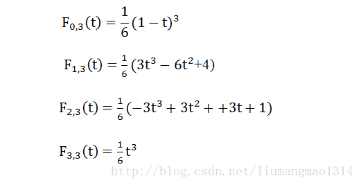
jerk就是对p(t)求三次导，这时会发现是一个常数，将每一段的jerk平方加起来，就得到cost。

梯度的求法：cost对控制点的求导。运用链式求导法则。

转变为cost对jerk的求导 * jerk对控制点的求导。

void BsplineOptimizer::calcSmoothnessCost(const vector<Eigen::Vector3d>& q, double& cost,
                                          vector<Eigen::Vector3d>& gradient) {
  cost = 0.0;
  Eigen::Vector3d zero(0, 0, 0);
  std::fill(gradient.begin(), gradient.end(), zero);
  Eigen::Vector3d jerk, temp_j;

  for (int i = 0; i < q.size() - order_; i++) {
    /* evaluate jerk */
    jerk = q[i + 3] - 3 * q[i + 2] + 3 * q[i + 1] - q[i];
    cost += jerk.squaredNorm();
    temp_j = 2.0 * jerk;
    /* jerk gradient */
    gradient[i + 0] += -temp_j;
    gradient[i + 1] += 3.0 * temp_j;
    gradient[i + 2] += -3.0 * temp_j;
    gradient[i + 3] += temp_j;
  }
}