《DSP using MATLAB》Problem 8.29

来汉有一月，往日的高温由于最近几个台风沿海登陆影响，今天终于下雨了，凉爽了几个小时。

接着做题。

%% ------------------------------------------------------------------------
%%            Output Info about this m-file
fprintf('\n***********************************************************\n');
fprintf('        <DSP using MATLAB> Problem 8.29 \n\n');

banner();
%% ------------------------------------------------------------------------

Fp = 1500;                    % analog passband freq in Hz
Fs = 2000;                    % analog stopband freq in Hz
fs = 8000;                    % sampling rate in Hz

% -------------------------------
%       ω = ΩT = 2πF/fs
% Digital Filter Specifications:
% -------------------------------
wp = 2*pi*Fp/fs;                 % digital passband freq in rad/sec
%wp = Fp;
ws = 2*pi*Fs/fs;                 % digital stopband freq in rad/sec
%ws = Fs;
Rp = 0.25;                        % passband ripple in dB
As = 80;                         % stopband attenuation in dB

Ripple = 10 ^ (-Rp/20)           % passband ripple in absolute
Attn = 10 ^ (-As/20)             % stopband attenuation in absolute

% Analog prototype specifications: Inverse Mapping for frequencies
T = 1/fs;                       % set T = 1
OmegaP = wp/T;               % prototype passband freq
OmegaS = ws/T;               % prototype stopband freq

% Analog Chebyshev-1 Prototype Filter Calculation:
[cs, ds] = afd_chb2(OmegaP, OmegaS, Rp, As);

% Calculation of second-order sections:
fprintf('\n***** Cascade-form in s-plane: START *****\n');
[CS, BS, AS] = sdir2cas(cs, ds)
fprintf('\n***** Cascade-form in s-plane: END *****\n');

% Calculation of Frequency Response:
[db_s, mag_s, pha_s, ww_s] = freqs_m(cs, ds, 2*pi/T);

% Calculation of Impulse Response:
[ha, x, t] = impulse(cs, ds);

% Match-z Transformation:
%[b, a] = imp_invr(cs, ds, T)        % digital Num and Deno coefficients of H(z)
[b, a] = mzt(cs, ds, T)            % digital Num and Deno coefficients of H(z)
[C, B, A] = dir2par(b, a)

% Calculation of Frequency Response:
[db, mag, pha, grd, ww] = freqz_m(b, a);

%% -----------------------------------------------------------------
%%                             Plot
%% -----------------------------------------------------------------
figure('NumberTitle', 'off', 'Name', 'Problem 8.29 Analog Chebyshev-2 lowpass')
set(gcf,'Color','white');
M = 1.2;                          % Omega max

subplot(2,2,1); plot(ww_s/(pi*1000), mag_s);  grid on; axis([-16, 16, 0, 1.1]);
xlabel(' Analog frequency in k\pi units'); ylabel('|H|'); title('Magnitude in Absolute');
set(gca, 'XTickMode', 'manual', 'XTick', [-2000, -1500, 0, 1500, 2000, 8000]*0.002);
set(gca, 'YTickMode', 'manual', 'YTick', [0, 0.0001, 0.5, 0.9716, 1]);

subplot(2,2,2); plot(ww_s/(pi*1000), db_s);  grid on; %axis([0, M, -50, 10]);
xlabel('Analog frequency in k\pi units'); ylabel('Decibels'); title('Magnitude in dB ');
set(gca, 'XTickMode', 'manual', 'XTick', [-2000, -1500, 0, 1500, 2000, 8000]*0.002);
set(gca, 'YTickMode', 'manual', 'YTick', [ -80, -1, 0]);
set(gca,'YTickLabelMode','manual','YTickLabel',['80';' 1';' 0']);

subplot(2,2,3); plot(ww_s/(pi*1000), pha_s/pi);  grid on; axis([-16, 16, -1.2, 1.2]);
xlabel('Analog frequency in k\pi nuits'); ylabel('radians'); title('Phase Response');
set(gca, 'XTickMode', 'manual', 'XTick', [-2000, -1500, 0, 1500, 2000, 8000]*0.002);
set(gca, 'YTickMode', 'manual', 'YTick', [-1:0.5:1]);

subplot(2,2,4); plot(t, ha); grid on; %axis([0, 30, -0.05, 0.25]);
xlabel('time in seconds'); ylabel('ha(t)'); title('Impulse Response');

figure('NumberTitle', 'off', 'Name', 'Problem 8.29 Digital Chebyshev-2 lowpass')
set(gcf,'Color','white');
M = 2;                          % Omega max

%%  Note  %%
%%  Magnitude of H(z) * T
%%  Note  %%
subplot(2,2,1); plot(ww/pi, mag/max(mag));  grid on; axis([0, M, 0, 1.1]);
xlabel(' frequency in \pi units'); ylabel('|H|'); title('Magnitude Response');
set(gca, 'XTickMode', 'manual', 'XTick', [0, 0.375, 0.5, 1.0, M]);
set(gca, 'YTickMode', 'manual', 'YTick', [0, 0.0001, 0.5, 0.9716, 1, 5, 10, 550]);

subplot(2,2,2); plot(ww/pi, pha/pi); axis([0, M, -1.1, 1.1]); grid on;
xlabel('frequency in \pi nuits'); ylabel('radians in \pi units'); title('Phase Response');
set(gca, 'XTickMode', 'manual', 'XTick', [0, 0.375, 0.5, 1.0, M]);
set(gca, 'YTickMode', 'manual', 'YTick', [-1:1:1]);

subplot(2,2,3); plot(ww/pi, db); axis([0, M, -120, 10]); grid on;
xlabel('frequency in \pi units'); ylabel('Decibels'); title('Magnitude in dB ');
set(gca, 'XTickMode', 'manual', 'XTick', [0, 0.375, 0.5, 1.0, M]);
set(gca, 'YTickMode', 'manual', 'YTick', [-80, -1, 0]);
set(gca,'YTickLabelMode','manual','YTickLabel',['80';' 1';' 0']);

subplot(2,2,4); plot(ww/pi, grd); grid on; %axis([0, M, 0, 35]);
xlabel('frequency in \pi units'); ylabel('Samples'); title('Group Delay');
set(gca, 'XTickMode', 'manual', 'XTick', [0, 0.375, 0.5, 1.0, M]);
%set(gca, 'YTickMode', 'manual', 'YTick', [0:5:35]);

figure('NumberTitle', 'off', 'Name', 'Problem 8.29 Pole-Zero Plot')
set(gcf,'Color','white');
zplane(b,a);
title(sprintf('Pole-Zero Plot'));
%pzplotz(b,a);

% Calculation of Impulse Response:
%[hs, xs, ts] = impulse(c, d);
figure('NumberTitle', 'off', 'Name', 'Problem 8.29 Imp & Freq Response')
set(gcf,'Color','white');
t = [0 : 0.000125 : 0.01]; subplot(2,1,1); impulse(cs,ds,t); grid on;   % Impulse response of the analog filter
axis([0, 0.01, -2000, 3000]);hold on

n = [0:1:0.01/T]; hn = filter(b,a,impseq(0,0,0.01/T));             % Impulse response of the digital filter
stem(n*T,hn); xlabel('time in sec'); title (sprintf('Impulse Responses, T=%f',T));
hold off

%n = [0:1:29];
%hz = impz(b, a, n);

% Calculation of Frequency Response:
[dbs, mags, phas, wws] = freqs_m(cs, ds, 2*pi/T);             % Analog frequency   s-domain  

[dbz, magz, phaz, grdz, wwz] = freqz_m(b, a);                 % Digital  z-domain

%% -----------------------------------------------------------------
%%                             Plot
%% -----------------------------------------------------------------  

M = 1/T;                          % Omega max

subplot(2,1,2); plot(wws/(2*pi),mags*Fs,'b', wwz/(2*pi)*Fs,magz,'r'); grid on;

xlabel('frequency in Hz'); title('Magnitude Responses'); ylabel('Magnitude'); 

text(1.4,.5,'Analog filter'); text(1.5,1.5,'Digital filter');

　　运行结果：

绝对指标

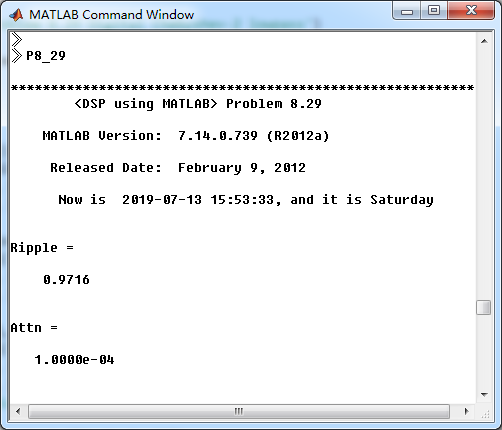
Chebyshev-2型模拟低通，系统函数串联形式系数

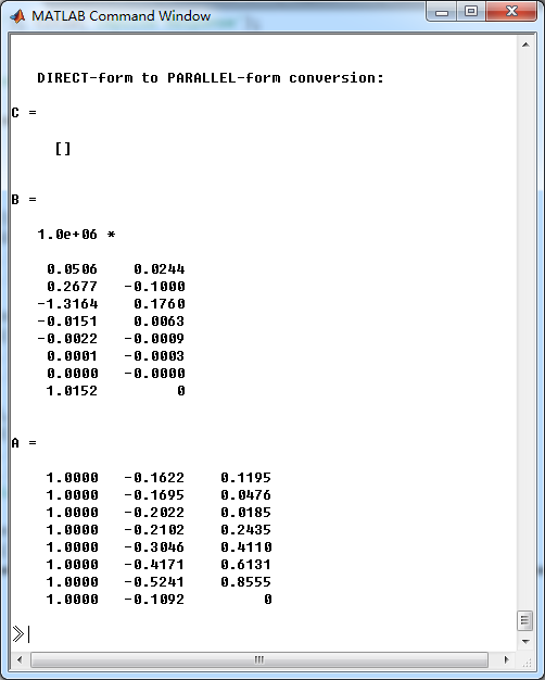
用match-z算法转换成数字低通，系统函数直接形式的系数

直接形式转换成并联形式，系数

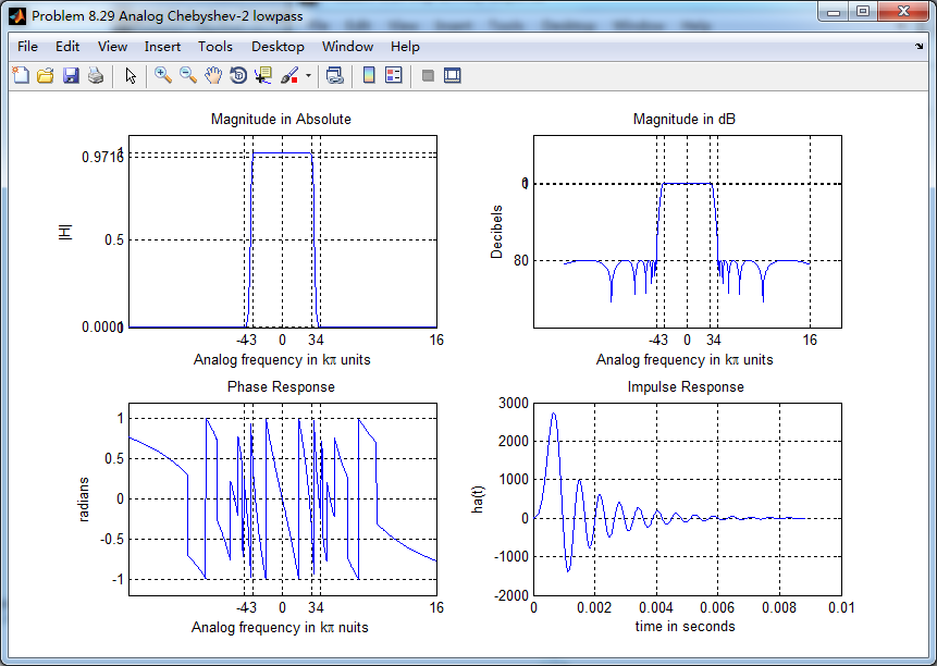
Chebyshev-2型模拟低通，幅度谱、相位谱和脉冲响应

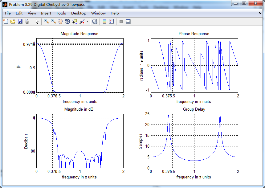
数字低通幅度谱、相位谱和群延迟响应

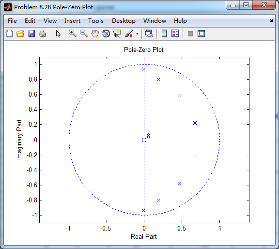
数字低通的零极点图

给定衰减值对应的精确频率值怎么求，暂时还不会，这里不计算了。