DeepLearning - Overview of Sequence model

I have had a hard time trying to understand recurrent model. Compared to Ng's deep learning course, I found Deep Learning book written by Ian, Yoshua and Aaron much easier to understand.

This post is structure in following order:

Intuitive interpretation of RNN
Basic RNN computation and different structure
RNN limitation and variants

Why we need Recurrent Neural Network

The main reason behind Convolution neural network is using sparse connection and parameter sharing to reduce the scale of NN. Then why we need recurrent neural network？

If we use traditional neural network to deal with a series input $(x^{<1>},x^{<2>},x^{<3>},..,x^{<t>})$, like speech, text, we will encounter 2 main challenges:

The input length varies. Of course we can cut or zero-pad the training data to have the same length. But how can we deal with the test data with unknown length?
For every time stamp, we will need a independent parameter. It makes it hard to capture the pattern in the sequence, compared to traditional time-series model like AR, ARIMA.

CNN can partly solve the second problem. By using a kernel with size K, the model can capture the pattern of k neighbors. Therefore, when the input length is fixed or limited, sometimes we do use CNN to deal with time-series data. However compared with sequence model, CNN has a very limited(shallow) parameter sharing. I will further talk about this below.

RNN Intuitive Interpretation

For a given sequence$(x^{<1>},x^{<2>},x^{<3>},..,x^{<t>})$, RNN takes in input in the following way:

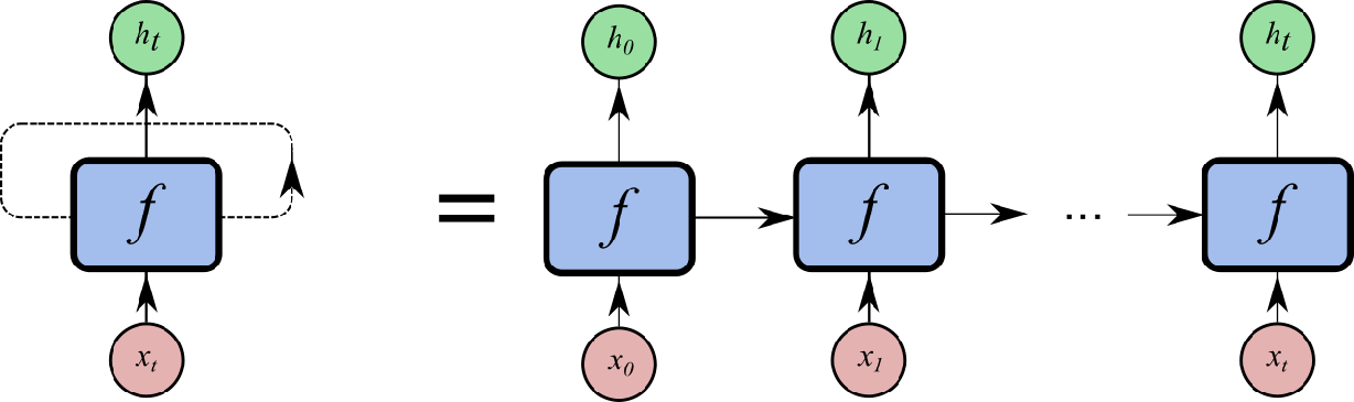
Regardless of how the output looks like, at each timestamp, the information is processed in the following way:
\[h^{<t>} = f(h^{<t-1>}, x^{<t>}, \theta)\]

I consider the above recurrent structure as having a neural network with unlimited number of hidden layer. Each hidden layer takes in information from input and previous hidden layer and they all share same parameter. The number of hidden layer is equal to your input length (time step).

There are 2 main advantages of above Recurrent structure:

The input size is fixed regardless of the the sequence length. Therefore it can be applied to any sequence without limitation.
- Case1: if the input is a multi-dimensional timeseries like open/high/low/close price in stock market, a 4-dimensional timeseries, then the input size is 4.
- Case2: if we use 10-dimensional vector to represent each word in sentence, then no matter how long the sentence is, the input size is 10.
Same parameter $\theta$ learnt at different timestamp. $\theta$ is not time-related, similar to the transformation matrix in Markov Chain.

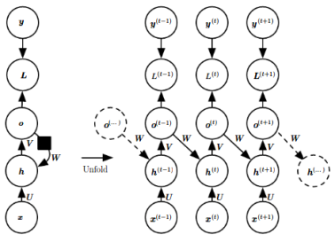
And if we further unfold the above formula, we will get following:
\[
\begin{align}
h^{<t>} & = f(h^{<t-1>}, x^{<t>}, \theta)
\\& = g^{<t>}(x^{<1>},x^{<2>},..,x^{<t>})
\end{align}
\]

Basically for hidden layer at time $t$, it can include all the information from the very beginning. Compared to Recurrent structure, CNN can only incorporate limited information from nearest K timestamp, where k is the kernel size.

Basic RNN Computation

Now let's add more details to basic RNN, below is the most representative structure of Basic RNN:

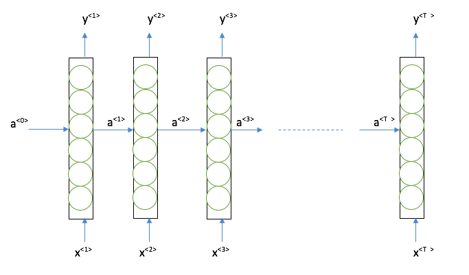
For each hidden layer, it takes both the information from input and the previous hidden layer,then generate an output. Since all the other format of RNN can be derived from this, we will go through the computation of RNN in above structure.

1. Forward propogation

Here I will mainly use the notation from Andrew's Course with small modification.
$a^{<t>}$ denotes the hidden layer output at time t
$x^{<t>}$ denotes the input at time t
$y^{<t>}$ denotes the target output at time t
$\hat{y}^{} $ denotes model output at time t
$o^{<t>}$ denotes the output before activation function.
$w_{aa}$, $w_{ax}$, $b_{a}$ are the weight and bias matrix at hidden layer
$w_{ya}$, $b_{y}$ are the weight and bias matrix used at output.

We will use $tanh$ activation function at hidden and $softmax$ at output.

For a given sample $( (x^{<1>},x^{<2>},..,x^{<T>} ), (y^{<1>},y^{<2>},..,y^{<T>} ) )$, RNN will start at time 0, and start forward propagation till T. At each time stamp t, following computation is made:
\[
\begin{align}
a^{<t>} &= tanh(w_{aa}a^{<t-1>} + w_{ax}x^{<t>} + b_{a})\\
o^{<t>} &= w_{ya}a^{<t>} + b{y} \\
\hat{y}^{<t>} &= softmax( o^{<t>} )
\end{align}
\]

We can further simplify the above formula by combining the weight matrix like below:
$W_a = [w_{aa}|w_{ax}]$, $[a^{<t-1>},x^{<t>}] = [\frac{a^{<t-1>}}{,x^{<t>}}]$

\[
\begin{align}
a^{<t>} = tanh(w_{a}[a^{<t-1>},x^{<t>}]+ b_{a}
\end{align}
\]
The negative log likelihood loss function of a sequence input is defined as following:
\[
\begin{align}
L({x^{<1>},..,x^{<T>}}, {y^{<1>},..,y^{<T>}}) & = \sum{L^{<t>}}
\\ & = -\sum{\log{p_{model}(y^{<t>}|x^{<1>},...,x^{<t>})}}
\end{align}
\]

2. Backward propagation

In recurrent neural network, same parameter is shared at different time. Therefore we need the gradient of all nodes to calculate the gradient of parameter. And don't forget that the gradient of each node not only takes information from output, but also from next hidden neuron. That's why Back-Propagation-through-time can not run parallel, but have to follow descending order of time.

Start from T, given loss function, and softmax activation function, gradient of $o^{<t>}$ is following:

\[
\begin{align}
\frac{\partial L}{\partial o^{<T>}} & = \frac{\partial L}{\partial L^{<T>}} \cdot
\frac{\partial L^{<T>}}{\partial \hat{y}^{<T>}} \cdot
\frac{\partial \hat{y}^{<T>}}{\partial {o}^{<T>}}
\\ & = 1 \cdot (-\frac{y^{<T>}}{\hat{y}^{<T>}} + \frac{1-y^{<T>}}{1-\hat{y}^{<T>}}) \cdot (\hat{y}^{<T>}(1-\hat{y}^{<T>}))
\\& = \hat{y}^{<T>}-y^{<T>}
\end{align}
\]
Therefroe we can get gradient of $a^{<T>}$ as below
\[
\begin{align}
\frac{\partial L}{\partial a^{<T>}} &=
\frac{\partial L}{\partial o^{<T>}} \cdot
\frac{\partial o^{<T>}}{\partial a^{<T>}}
\\& = W_{ya}^T \cdot \frac{\partial L}{\partial o^{<T>}}
\end{align}
\]
For the last node, the gradient only consider $o^{<T>}$, while for all the other nodes, the gradient need to consider both $o^{<t>}$ and $a^{<t+1>}$, we will get following:
\[
\begin{align}
\frac{\partial L}{\partial a^{<t>}} &=
\frac{\partial L}{\partial o^{<t>}} \cdot
\frac{\partial o^{<t>}}{\partial a^{<t>}} +
\frac{\partial L}{\partial a^{<t+1>}} \cdot
\frac{\partial a^{<t+1>}}{\partial a^{<t>}}
\\ & = W_{ya}^T \cdot \frac{\partial L}{\partial o^{<t>}} + W_{aa}^T \cdot diag(1-(a^{<t+1>})^2) \cdot \frac{\partial L}{\partial a^{<t+1>}}
\end{align}
\]

Now we have the gradient for each hidden neuron, we can further get the gradient for all the parameter, given that same parameters are shared at different time stamp. see below:
\[
\begin{align}
\frac{\partial L}{\partial b_y} &= \sum_t{\frac{\partial L}{\partial o^{<t>}} }\\
\frac{\partial L}{\partial b_a} &= \sum_t{ diag(1-(a^{<t>})^2) \cdot \frac{\partial L}{\partial a^{<t>}} } \\
\frac{\partial L}{\partial w_{ya}} &= \sum_t{ \frac{\partial L}{\partial o^{<t>}} \cdot {a^{<t>}}^T } \\
\frac{\partial L}{\partial w_{aa}} &= \sum_t{ \frac{\partial L}{\partial a^{<t>}} \cdot diag(1-(a^{<t>})^2) \cdot {a^{<t-1>}}^T } \\
\frac{\partial L}{\partial w_{ax}} &= \sum_t{ \frac{\partial L}{\partial a^{<t>}} \cdot diag(1-(a^{<t>})^2) \cdot {x^{<t>}}^T } \\
\end{align}
\]

3. Different structures of RNN

So far the RNN we have talked about has 2 main features: input length = output length, and direct connection between hidden neuron. While actually RNN have many variants. We can further classify the difference as following:

How recurrent works
Different input and output length

As for how recurrent works, there are 2 basic types:

there is recurrent connection between hidden neuron, see below RNN1
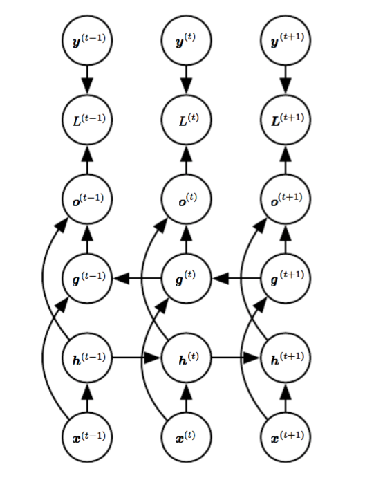
there is recurrent connection between output and hidden neuron, see below RNN2

RNN1. Hidden to Hidden

RNN2. Ouput to Hidden

Apparently Hidden to Hidden Recurrent will contain more information about the history. Because output at each timestamp is optimized to simulate the target output, it can't have as much information as its hidden neuron.

Then why we need the second type, since it loses information in propagation. To answer to this we will have to talk about BPTT - Back Propagation Through Time. Due to the recurrent structure, we have to process hidden layer one after another in both forward and backward propagation. Therefore both memory usage and computation time is O(T) and we can't use parallel computation to speed up.

To be able to use parallel computation, we have to disconnect history and present while still using the information from past. One solution is a derived type of Output to hidden recurrent - Teacher forcing. Basically it passes the realized output instead of estimated output to the next hidden neuron. Like below:

Teacher forcing Train & Test

It changes the original maximum log likelihood into conditional log likelihood.
\[
\begin{align}
& p(y^{(1)},y^{(2)}|x^{(1)},x^{(2)})
\\ &= p(y^{(1)}|X^{(1)},X^{(2)}) + p(y^{(1)}|y^{(1)}, X^{(1)},y^{(1)})
\end{align}
\]

However teacher forcing has a big problem that the input distribution of training and testing is different, since we don't have realized output in testing. Later we will talk about how to overcome such problem.

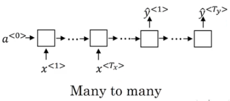
Next Let's talk about input and output length. In the below image, it gives all the possibilities:

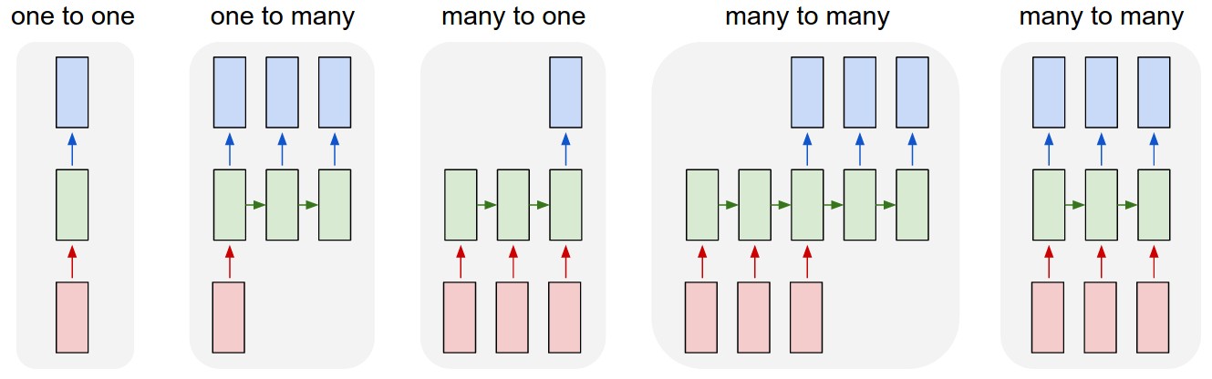
many-to-many(seq2seq) with same length is the one we have been talking so far. Let' go through others.

many-to-one(seq2one) can be used in sentiment analysis. The only difference between the RNN we have been talking about and many-to-one is that each sequence input has only 1 ouput.

one-to-many(one2seq) can be used in music generation. It uses the second recurrent structure - feeding output to next hidden neuron.

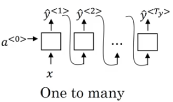
many-to-many(seq2seq) with different length is wildly known as Encoder-Decoder System. It has many application in machine translation due to its flexibility. We will further talk about this in the application post.

Basic RNN limitation and variants

Now we see what basic RNN can do. Dose it has any limitation? And how do we get around with it?

1. Time order - Bidirection RNN

We have been emphasizing that RNN has to compute in order of time in propagation, meaning the $\hat{y}^{<t>}$ is only based on the information prior from $x^{<1>}$ to $x^{<t>}$. However there are situations that we need to consider both prior and post information, for example in translation we need to consider the entire context. Like following:

2. long-term dependence

We have mentioned the gradient vanishing/exploding problem before for deep neural network. Same idea also applies here. In Deep Learning book, author gives an intuitive explanation.

If we consider a simplified RNN without input $x$ and activation function. Then RNN becomes a time-series model with matrix implementation as following:
\[
\begin{align}
a^{<t>} & = ({W_{aa}}^t)^T \cdot a^{<0>} \\
where \ \ \ \
W_{aa} &= Q \Lambda Q^T \\
Then \ \ \ \
a^{<t>} & = Q {\Lambda}^t Q^T\cdot a^{<0>}
\end{align}
\]
The problem lies in Eigenvalue ${\Lambda}^t$, where $\lambda >1$ may lead to gradient exploding, while $\lambda <1$ may lead to gradient vanishing.

Gradient exploding can be solved by gradient clipping. Basically we cap the gradient for certain threshold. For gradient vanishing, one popular solution is gated RNN. Gated model has additional parameter to control at each timestamp whether to remember or forget the pass information, in order to maintain useful information for longer time period.

Gated RNN 1 - GRU Unit

Based on basic RNN, GRU add more computation within in each hidden neuron to control information flow. We use $c^{<t>}$ to denote hidden layer output. And within each hidden layer, we do following:
\[
\begin{align}
\Gamma_u & =\sigma(w_{u}[c^{<t-1>},x^{<t>}]+ b_{u})\\
\Gamma_r & =\sigma(w_{r}[c^{<t-1>},x^{<t>}]+ b_{r})\\
\tilde{c}^{<t>} &= tanh( w_{a}[ \Gamma_r \odot c^{<t-1>},x^{<t>}]+ b_{a} )\\
c^{<t>} &= \Gamma_u \odot \tilde{c}^{<t>} + (1-\Gamma_u) \odot
\tilde{c}^{<t-1>}
\end{align}
\]

Where $\Gamma_u$ is the update Gate, and $\Gamma_r$ is the reset gate. They both measure the relevance between the previous hidden layer and the present input. Please note here $\Gamma_r$ and $\Gamma_u$ has same dimension as $c^{<t>}$, and element-wise multiplication is applied.

If the relevance is low than update gate $\Gamma_u$ will choose to forget history information,and reset gate $\Gamma_r$ will also allow less history information into the current calculation. If $\Gamma_r=1$ and $\Gamma_u=0$ then we get basic RNN.

And sometimes only $\Gamma_u$ is used, leading to a simplified GRU with less parameter to train.

Gated RNN 2 - LSTM Unit

Another solution to long-term dependence is LSTM unit. It has 3 gates to train.
\[
\begin{align}
\Gamma_u & =\sigma(w_{u}[c^{<t-1>},x^{<t>}]+ b_{u})\\
\Gamma_f & =\sigma(w_{f}[c^{<t-1>},x^{<t>}]+ b_{f})\\
\Gamma_o & =\sigma(w_{o}[c^{<t-1>},x^{<t>}]+ b_{o})\\
\tilde{c}^{<t>} &= tanh( w_{a}[ c^{<t-1>},x^{<t>}]+ b_{a} )\\
c^{<t>} &= \Gamma_u \odot \tilde{c}^{<t>} + \Gamma_f \odot
\tilde{c}^{<t-1>}\\
a^{<t>} &= \Gamma_o \odot tanh(c^{<t>} )
\end{align}
\]

Where $\Gamma_u$ is the update Gate, and $\Gamma_f$ is the forget gate, and $\Gamma_o$ is the output gate.

Beside GRU and LSTM, there are also other variants. It is hard to say which is the best. If your data set is small, maybe you should try simplified RNN, instead of LSTM, which has less parameter to train.

So far we have reviewed most of the basic knowledge in Neural Network. Let's have some fun in the next post. The next post for this series will be some cool applications in CNN and RNN.

To be continued.

Reference

Ian Goodfellow, Yoshua Bengio, Aaron Conrville, "Deep Learning"
Bishop, "Pattern Recognition and Machine Learning",springer, 2006
T. Hastie, R. Tibshirani and J. Friedman. “Elements of Statistical Learning”, Springer, 2009.