python机器学习——使用scikit-learn训练感知机模型

这一篇我们将开始使用scikit-learn的API来实现模型并进行训练，这个包大大方便了我们的学习过程，其中包含了对常用算法的实现，并进行高度优化，以及含有数据预处理、调参和模型评估的很多方法。

我们来看一个之前看过的实例，不过这次我们使用sklearn来训练一个感知器模型，数据集还是Iris，使用其中两维度的特征，样本数据使用三个类别的全部150个样本

%matplotlib inline
import numpy as np
from sklearn import datasets

iris = datasets.load_iris()
X = iris.data[:, [2, 3]]
y = iris.target

np.unique(y)

array([0, 1, 2])

为了评估训练好的模型对新数据的预测能力，我们这里将Iris数据集分为训练集和测试集，这里我们通过调用trian_test_split方法来将数据集分为两部分，其中测试集占30%，训练集占70%

from sklearn.model_selection import train_test_split
X_train, X_test, y_train, y_test = train_test_split(X, y, test_size=0.3, random_state=0)

我们再将特征进行缩放操作，这里调用StandardScaler来对特征进行标准化：

from sklearn.preprocessing import StandardScaler
sc = StandardScaler()
sc.fit(X_train)
X_train_std = sc.transform(X_train)
X_test_std = sc.transform(X_test)

新对象sc使用fit方法对数据集中每一维的特征计算出样本平均值和标准差，然后调用transform方法对数据集进行标准化，我们这里使用相同的标准化参数对待训练集和测试集。接下来我们训练一个感知器模型

from sklearn.linear_model import Perceptron

ppn = Perceptron(max_iter=40, eta0=0.1, random_state=0)

ppn.fit(X_train_std, y_train)

Perceptron(alpha=0.0001, class_weight=None, early_stopping=False, eta0=0.1,
           fit_intercept=True, max_iter=40, n_iter_no_change=5, n_jobs=None,
           penalty=None, random_state=0, shuffle=True, tol=0.001,
           validation_fraction=0.1, verbose=0, warm_start=False)

y_pred = ppn.predict(X_test_std)

print('Misclassified samples: %d' % (y_test != y_pred).sum())

Misclassified samples: 5

可以看出测试集中有5个样本被分错类了，因此错误分类率是0.11，则分类准确率为1-0.11=0.89，我们也可以直接计算分类准确率：

from sklearn.metrics import accuracy_score

print('Accuracy: %.2f' % accuracy_score(y_test, y_pred))

Accuracy: 0.89

最后我们画出分界区域,这里我们将plot_decision_regions函数进行一些修改，使我们可以区分训练集和测试集的样本

from matplotlib.colors import ListedColormap
import matplotlib.pyplot as plt

def plot_decision_regions(X, y, classifier, test_idx=None, resolution=0.02):
    # setup marker generator and color map
    markers = ('s', 'x', 'o', '^', 'v')
    colors = ('red', 'blue', 'lightgreen', 'gray', 'cyan')
    cmap = ListedColormap(colors[:len(np.unique(y))])

    # plot the decision surface
    x1_min, x1_max = X[:, 0].min() - 1, X[:, 0].max() + 1
    x2_min, x2_max = X[:, 1].min() - 1, X[:, 1].max() + 1
    xx1, xx2 = np.meshgrid(np.arange(x1_min, x1_max, resolution),
                          np.arange(x2_min, x2_max, resolution))
    Z = classifier.predict(np.array([xx1.ravel(), xx2.ravel()]).T)
    Z = Z.reshape(xx1.shape)
    plt.contourf(xx1, xx2, Z, slpha=0.4, cmap=cmap)
    plt.xlim(xx1.min(), xx1.max())
    plt.ylim(xx2.min(), xx2.max())

    # plot all samples
    X_test, y_test = X[test_idx, :], y[test_idx]
    for idx, cl in enumerate(np.unique(y)):
        plt.scatter(x=X[y == cl, 0], y=X[y == cl, 1], alpha=0.8,
                   c=cmap(idx), marker=markers[idx], label=cl)

    # highlight test samples
    if test_idx:
        X_test, y_test = X[test_idx, :], y[test_idx]
        plt.scatter(X_test[:, 0], X_test[:, 1], c='',alpha=1.0,
                   linewidth=1, marker='o', s=55, label='test set')

X_combined_std = np.vstack((X_train_std, X_test_std))

y_combined = np.hstack((y_train, y_test))

plot_decision_regions(X=X_combined_std, y=y_combined, classifier=ppn,
                     test_idx=range(105, 150))
plt.xlabel('petal length [standardized]')
plt.ylabel('petal width [standardized]')
plt.legend(loc='upper left')
plt.show()

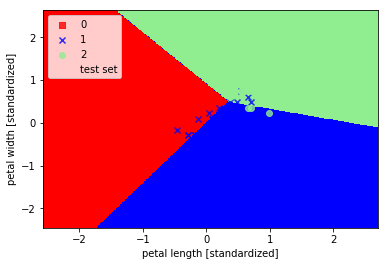
可以看出三个类别并没有被完美分类，这是由于这三类花并不是线性可分的数据。