吴裕雄 python 机器学习——支持向量机SVM非线性分类SVC模型

import numpy as np
import matplotlib.pyplot as plt

from sklearn import datasets, linear_model,svm
from sklearn.model_selection import train_test_split

def load_data_classfication():
    '''
    加载用于分类问题的数据集
    '''
    # 使用 scikit-learn 自带的 iris 数据集
    iris=datasets.load_iris()
    X_train=iris.data
    y_train=iris.target
    # 分层采样拆分成训练集和测试集，测试集大小为原始数据集大小的 1/4
    return train_test_split(X_train, y_train,test_size=0.25,random_state=0,stratify=y_train) 

#支持向量机SVM非线性分类SVC模型
def test_SVC_linear(*data):
    X_train,X_test,y_train,y_test=data
    cls=svm.SVC(kernel='linear')
    cls.fit(X_train,y_train)
    print('Coefficients:%s, intercept %s'%(cls.coef_,cls.intercept_))
    print('Score: %.2f' % cls.score(X_test, y_test))

# 生成用于分类的数据集
X_train,X_test,y_train,y_test=load_data_classfication()
# 调用 test_SVC_linear
test_SVC_linear(X_train,X_test,y_train,y_test) 

def test_SVC_poly(*data):
    '''
    测试多项式核的 SVC 的预测性能随 degree、gamma、coef0 的影响.
    '''
    X_train,X_test,y_train,y_test=data
    fig=plt.figure()
    ### 测试 degree ####
    degrees=range(1,20)
    train_scores=[]
    test_scores=[]
    for degree in degrees:
        cls=svm.SVC(kernel='poly',degree=degree)
        cls.fit(X_train,y_train)
        train_scores.append(cls.score(X_train,y_train))
        test_scores.append(cls.score(X_test, y_test))
    ax=fig.add_subplot(1,3,1) # 一行三列
    ax.plot(degrees,train_scores,label="Training score ",marker='+' )
    ax.plot(degrees,test_scores,label= " Testing  score ",marker='o' )
    ax.set_title( "SVC_poly_degree ")
    ax.set_xlabel("p")
    ax.set_ylabel("score")
    ax.set_ylim(0,1.05)
    ax.legend(loc="best",framealpha=0.5)

    ### 测试 gamma ，此时 degree 固定为 3####
    gammas=range(1,20)
    train_scores=[]
    test_scores=[]
    for gamma in gammas:
        cls=svm.SVC(kernel='poly',gamma=gamma,degree=3)
        cls.fit(X_train,y_train)
        train_scores.append(cls.score(X_train,y_train))
        test_scores.append(cls.score(X_test, y_test))
    ax=fig.add_subplot(1,3,2)
    ax.plot(gammas,train_scores,label="Training score ",marker='+' )
    ax.plot(gammas,test_scores,label= " Testing  score ",marker='o' )
    ax.set_title( "SVC_poly_gamma ")
    ax.set_xlabel(r"$\gamma$")
    ax.set_ylabel("score")
    ax.set_ylim(0,1.05)
    ax.legend(loc="best",framealpha=0.5)
    ### 测试 r ，此时 gamma固定为10 ， degree 固定为 3######
    rs=range(0,20)
    train_scores=[]
    test_scores=[]
    for r in rs:
        cls=svm.SVC(kernel='poly',gamma=10,degree=3,coef0=r)
        cls.fit(X_train,y_train)
        train_scores.append(cls.score(X_train,y_train))
        test_scores.append(cls.score(X_test, y_test))
    ax=fig.add_subplot(1,3,3)
    ax.plot(rs,train_scores,label="Training score ",marker='+' )
    ax.plot(rs,test_scores,label= " Testing  score ",marker='o' )
    ax.set_title( "SVC_poly_r ")
    ax.set_xlabel(r"r")
    ax.set_ylabel("score")
    ax.set_ylim(0,1.05)
    ax.legend(loc="best",framealpha=0.5)
    plt.show()

# 调用 test_SVC_poly
test_SVC_poly(X_train,X_test,y_train,y_test) 

def test_SVC_rbf(*data):
    '''
    测试 高斯核的 SVC 的预测性能随 gamma 参数的影响
    '''
    X_train,X_test,y_train,y_test=data
    gammas=range(1,20)
    train_scores=[]
    test_scores=[]
    for gamma in gammas:
        cls=svm.SVC(kernel='rbf',gamma=gamma)
        cls.fit(X_train,y_train)
        train_scores.append(cls.score(X_train,y_train))
        test_scores.append(cls.score(X_test, y_test))
    fig=plt.figure()
    ax=fig.add_subplot(1,1,1)
    ax.plot(gammas,train_scores,label="Training score ",marker='+' )
    ax.plot(gammas,test_scores,label= " Testing  score ",marker='o' )
    ax.set_title( "SVC_rbf")
    ax.set_xlabel(r"$\gamma$")
    ax.set_ylabel("score")
    ax.set_ylim(0,1.05)
    ax.legend(loc="best",framealpha=0.5)
    plt.show()

# 调用 test_SVC_rbf
test_SVC_rbf(X_train,X_test,y_train,y_test) 

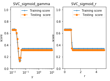
def test_SVC_sigmoid(*data):
    '''
    测试 sigmoid 核的 SVC 的预测性能随 gamma、coef0 的影响.
    '''
    X_train,X_test,y_train,y_test=data
    fig=plt.figure()

    ### 测试 gamma ，固定 coef0 为 0 ####
    gammas=np.logspace(-2,1)
    train_scores=[]
    test_scores=[]

    for gamma in gammas:
        cls=svm.SVC(kernel='sigmoid',gamma=gamma,coef0=0)
        cls.fit(X_train,y_train)
        train_scores.append(cls.score(X_train,y_train))
        test_scores.append(cls.score(X_test, y_test))
    ax=fig.add_subplot(1,2,1)
    ax.plot(gammas,train_scores,label="Training score ",marker='+' )
    ax.plot(gammas,test_scores,label= " Testing  score ",marker='o' )
    ax.set_title( "SVC_sigmoid_gamma ")
    ax.set_xscale("log")
    ax.set_xlabel(r"$\gamma$")
    ax.set_ylabel("score")
    ax.set_ylim(0,1.05)
    ax.legend(loc="best",framealpha=0.5)
    ### 测试 r，固定 gamma 为 0.01 ######
    rs=np.linspace(0,5)
    train_scores=[]
    test_scores=[]

    for r in rs:
        cls=svm.SVC(kernel='sigmoid',coef0=r,gamma=0.01)
        cls.fit(X_train,y_train)
        train_scores.append(cls.score(X_train,y_train))
        test_scores.append(cls.score(X_test, y_test))
    ax=fig.add_subplot(1,2,2)
    ax.plot(rs,train_scores,label="Training score ",marker='+' )
    ax.plot(rs,test_scores,label= " Testing  score ",marker='o' )
    ax.set_title( "SVC_sigmoid_r ")
    ax.set_xlabel(r"r")
    ax.set_ylabel("score")
    ax.set_ylim(0,1.05)
    ax.legend(loc="best",framealpha=0.5)
    plt.show()

# 调用 test_SVC_sigmoid
test_SVC_sigmoid(X_train,X_test,y_train,y_test)