scikit-learn画ROC图

1.使用sklearn库和matplotlib.pyplot库

import sklearn
import matplotlib.pyplot as plt

2.准备绘图函数的传入参数1.预测的概率值数组2.预测的labels值数组

for i in range(len(y_labeles)):
    a = np.argmax(y_labeles[i])
    y_pred.append(y_conv.eval(feed_dict={x: np.reshape(mnist.test.images[i], [1, 784]),  keep_prob: 0.5}, session=sess)[0][a])
    y_labeles_d1.append(correct_prediction.eval(feed_dict={x: np.reshape(mnist.test.images[i], [1, 784]), y_: np.reshape(y_labeles[i], [1, 10]), keep_prob: 0.5}, session=sess))

3.调用sklearn.metrics.roc_curve();

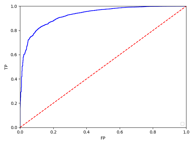
fpr, tpr, thresholds = sklearn.metrics.roc_curve(y_labeles_d1, y_pred)

plt.plot(fpr, tpr, 'b')#生成ROC曲线
plt.legend(loc='lower right')
plt.plot([0, 1], [0, 1], 'r--')
plt.xlim([0, 1])
plt.ylim([0, 1])
plt.ylabel('TP')
plt.xlabel('FP')
plt.show()

4.例子

import tensorflow as tf
from tensorflow.examples.tutorials.mnist import input_data
import numpy as np
import sklearn
import matplotlib.pyplot as plt

mnist = input_data.read_data_sets('data/', one_hot=True)

def weight_variable(shape, name):
    initial = tf.truncated_normal(shape, stddev=0.1, name=name)
    return tf.Variable(initial)

def bias_variable(shape, name):
    initial = tf.constant(0.1, shape=shape, name=name)
    return tf.Variable(initial)

def conv2d(x, W):
    return tf.nn.conv2d(x, W, strides=[1, 1, 1, 1], padding='SAME')

def max_pool_2x2(x):
    return tf.nn.max_pool(x, ksize=[1, 2, 2, 1], strides=[1, 2, 2, 1], padding='SAME')

x = tf.placeholder(tf.float32, [None, 784])
y_ = tf.placeholder(tf.float32, [None, 10])
x_image = tf.reshape(x, [-1, 28, 28, 1])

W_conv1 = weight_variable([5, 5, 1, 32], name='W_conv1')
b_conv1 = bias_variable([32], name='b_conv1')
h_conv1 = tf.nn.relu(conv2d(x_image, W_conv1) + b_conv1)
h_pool1 = max_pool_2x2(h_conv1)

W_conv2 = weight_variable([5, 5, 32, 64], name='W_conv2')
b_conv2 = bias_variable([64], name='b_conv2')
h_conv2 = tf.nn.relu(conv2d(h_pool1, W_conv2) + b_conv2)
h_pool2 = max_pool_2x2(h_conv2)

W_fc1 = weight_variable([7*7*64, 1024], name='W_fc1')
b_fc1 = bias_variable([1024], name='b_fc1')
h_pool2_flat = tf.reshape(h_pool2, [-1, 7*7*64])
h_fc1 = tf.nn.relu(tf.matmul(h_pool2_flat, W_fc1) + b_fc1)

keep_prob = tf.placeholder(tf.float32)
h_fc1_drop = tf.nn.dropout(h_fc1, keep_prob)

W_fc2 = weight_variable([1024, 10], name='W_fc2')
b_fc2 = bias_variable([10], name='b_fc2')
y_conv = tf.nn.softmax(tf.matmul(h_fc1_drop, W_fc2) + b_fc2)

cross_entropy = tf.reduce_sum(tf.nn.softmax_cross_entropy_with_logits(logits=y_conv, labels=y_))

# cross_entropy = tf.reduce_mean(-tf.reduce_sum(y_ * tf.log(y_conv), reduction_indices=[1]))
train_step = tf.train.AdamOptimizer(1e-4).minimize(cross_entropy)

correct_prediction = tf.equal(tf.argmax(y_conv, 1), tf.argmax(y_, 1))
accuracy = tf.reduce_mean(tf.cast(correct_prediction, tf.float32))

sess = tf.Session()
sess.run(tf.global_variables_initializer())

for i in range(500):

    batch = mnist.train.next_batch(100)

    train_step.run(session=sess, feed_dict={x: batch[0], y_: batch[1], keep_prob: 0.5})
    if i % 500 == 0 and i != 0:
        train_accuracy = accuracy.eval(session=sess, feed_dict={x: batch[0], y_: batch[1], keep_prob: 1.0})
        print('step %d, training accuracy %g' % (i, train_accuracy))

print("!!!!!")
print('test accuracy %g' % accuracy.eval(session=sess, feed_dict={
    x: mnist.test.images, y_: mnist.test.labels, keep_prob: 1.0
}))

saver = tf.train.Saver()
saver.save(sess, './trained_variables.ckpt', global_step=1000)

y_labeles = mnist.test.labels
y_pred = []
y_labeles_d1 = []

for i in range(len(y_labeles)):
    a = np.argmax(y_labeles[i])
    y_pred.append(y_conv.eval(feed_dict={x: np.reshape(mnist.test.images[i], [1, 784]),  keep_prob: 0.5}, session=sess)[0][a])
    y_labeles_d1.append(correct_prediction.eval(feed_dict={x: np.reshape(mnist.test.images[i], [1, 784]), y_: np.reshape(y_labeles[i], [1, 10]), keep_prob: 0.5}, session=sess))

fpr, tpr, thresholds = sklearn.metrics.roc_curve(y_labeles_d1, y_pred)

plt.plot(fpr, tpr, 'b')#生成ROC曲线
plt.legend(loc='lower right')
plt.plot([0, 1], [0, 1], 'r--')
plt.xlim([0, 1])
plt.ylim([0, 1])
plt.ylabel('TP')
plt.xlabel('FP')
plt.show()

# with tf.Session() as sess:
#   new_saver = tf.train.import_meta_graph('my_test_model-1000.meta')
#   new_saver.restore(sess, tf.train.latest_checkpoint('./'))

# print(sess.run(W_conv1))

5.效果：