Seaborn线性关系数据可视化

regplot()

绘制两个变量的线性拟合图。

sns.regplot(
    x,
    y,
    data=None,
    x_estimator=None,
    x_bins=None,
    x_ci='ci',
    scatter=True,
    fit_reg=True,
    ci=95,
    n_boot=1000,
    units=None,
    order=1,
    logistic=False,
    lowess=False,
    robust=False,
    logx=False,
    x_partial=None,
    y_partial=None,
    truncate=False,
    dropna=True,
    x_jitter=None,
    y_jitter=None,
    label=None,
    color=None,
    marker='o',
    scatter_kws=None,
    line_kws=None,
    ax=None,
)
Docstring:
Plot data and a linear regression model fit.

There are a number of mutually exclusive options for estimating the
regression model. See the :ref:`tutorial <regression_tutorial>` for more
information.    

Parameters
----------
x, y: string, series, or vector array
    Input variables. If strings, these should correspond with column names
    in ``data``. When pandas objects are used, axes will be labeled with
    the series name.
data : DataFrame
    Tidy ("long-form") dataframe where each column is a variable and each
    row is an observation.
x_estimator : callable that maps vector -> scalar, optional
    Apply this function to each unique value of ``x`` and plot the
    resulting estimate. This is useful when ``x`` is a discrete variable.
    If ``x_ci`` is given, this estimate will be bootstrapped and a
    confidence interval will be drawn.
x_bins : int or vector, optional
    Bin the ``x`` variable into discrete bins and then estimate the central
    tendency and a confidence interval. This binning only influences how
    the scatterplot is drawn; the regression is still fit to the original
    data.  This parameter is interpreted either as the number of
    evenly-sized (not necessary spaced) bins or the positions of the bin
    centers. When this parameter is used, it implies that the default of
    ``x_estimator`` is ``numpy.mean``.
x_ci : "ci", "sd", int in [0, 100] or None, optional
    Size of the confidence interval used when plotting a central tendency
    for discrete values of ``x``. If ``"ci"``, defer to the value of the
    ``ci`` parameter. If ``"sd"``, skip bootstrapping and show the
    standard deviation of the observations in each bin.
scatter : bool, optional
    If ``True``, draw a scatterplot with the underlying observations (or
    the ``x_estimator`` values).
fit_reg : bool, optional
    If ``True``, estimate and plot a regression model relating the ``x``
    and ``y`` variables.
ci : int in [0, 100] or None, optional
    Size of the confidence interval for the regression estimate. This will
    be drawn using translucent bands around the regression line. The
    confidence interval is estimated using a bootstrap; for large
    datasets, it may be advisable to avoid that computation by setting
    this parameter to None.
n_boot : int, optional
    Number of bootstrap resamples used to estimate the ``ci``. The default
    value attempts to balance time and stability; you may want to increase
    this value for "final" versions of plots.
units : variable name in ``data``, optional
    If the ``x`` and ``y`` observations are nested within sampling units,
    those can be specified here. This will be taken into account when
    computing the confidence intervals by performing a multilevel bootstrap
    that resamples both units and observations (within unit). This does not
    otherwise influence how the regression is estimated or drawn.
order : int, optional
    If ``order`` is greater than 1, use ``numpy.polyfit`` to estimate a
    polynomial regression.
logistic : bool, optional
    If ``True``, assume that ``y`` is a binary variable and use
    ``statsmodels`` to estimate a logistic regression model. Note that this
    is substantially more computationally intensive than linear regression,
    so you may wish to decrease the number of bootstrap resamples
    (``n_boot``) or set ``ci`` to None.
lowess : bool, optional
    If ``True``, use ``statsmodels`` to estimate a nonparametric lowess
    model (locally weighted linear regression). Note that confidence
    intervals cannot currently be drawn for this kind of model.
robust : bool, optional
    If ``True``, use ``statsmodels`` to estimate a robust regression. This
    will de-weight outliers. Note that this is substantially more
    computationally intensive than standard linear regression, so you may
    wish to decrease the number of bootstrap resamples (``n_boot``) or set
    ``ci`` to None.
logx : bool, optional
    If ``True``, estimate a linear regression of the form y ~ log(x), but
    plot the scatterplot and regression model in the input space. Note that
    ``x`` must be positive for this to work.
{x,y}_partial : strings in ``data`` or matrices
    Confounding variables to regress out of the ``x`` or ``y`` variables
    before plotting.
truncate : bool, optional
    By default, the regression line is drawn to fill the x axis limits
    after the scatterplot is drawn. If ``truncate`` is ``True``, it will
    instead by bounded by the data limits.
{x,y}_jitter : floats, optional
    Add uniform random noise of this size to either the ``x`` or ``y``
    variables. The noise is added to a copy of the data after fitting the
    regression, and only influences the look of the scatterplot. This can
    be helpful when plotting variables that take discrete values.
label : string
    Label to apply to ether the scatterplot or regression line (if
    ``scatter`` is ``False``) for use in a legend.
color : matplotlib color
    Color to apply to all plot elements; will be superseded by colors
    passed in ``scatter_kws`` or ``line_kws``.
marker : matplotlib marker code
    Marker to use for the scatterplot glyphs.
{scatter,line}_kws : dictionaries
    Additional keyword arguments to pass to ``plt.scatter`` and
    ``plt.plot``.
ax : matplotlib Axes, optional
    Axes object to draw the plot onto, otherwise uses the current Axes.

Returns
-------
ax : matplotlib Axes
    The Axes object containing the plot.

See Also
--------
lmplot : Combine :func:`regplot` and :class:`FacetGrid` to plot multiple
         linear relationships in a dataset.
jointplot : Combine :func:`regplot` and :class:`JointGrid` (when used with
            ``kind="reg"``).
pairplot : Combine :func:`regplot` and :class:`PairGrid` (when used with
           ``kind="reg"``).
residplot : Plot the residuals of a linear regression model.

#设置风格
sns.set_style('whitegrid')
#导入数据
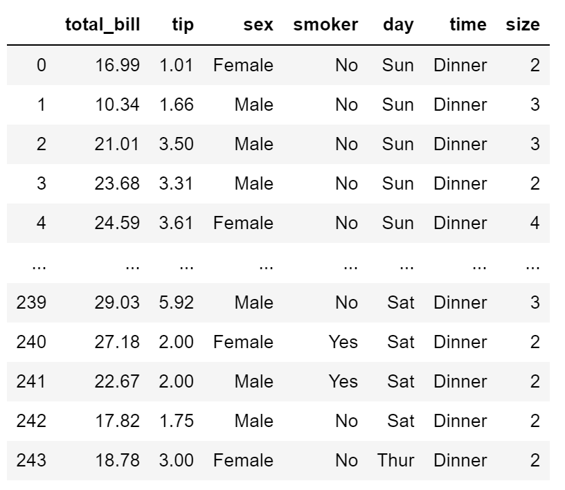
tips = sns.load_dataset('tips', data_home='seaborn-data')
tips

#回归图
#regplot()
ax = sns.regplot(x='total_bill', y='tip', data=tips)

#离散回归图
ax = sns.regplot(x='size', y='total_bill', data=tips)

#离散回归图
#x_estimator设置离散数据显示的方式（mean表示平均值），ci置信区间默认95%
ax = sns.regplot(x='size', y='total_bill', data=tips, x_estimator=np.mean)

#创建正态分布的数组
np.random.seed(8)
mean = (4, 6)
cov = [[1.5,0.7], [0.7,1]]
x,y = np.random.multivariate_normal(mean, cov, 100).T
#绘制回归图
ax= sns.regplot(x=x, y=y, color='g')

#ci设置置信区间（68表示68%）
ax = sns.regplot(x=x, y=y, ci=68)

#robust设置稳健回归，ci=None设置不显示置信区间
ax = sns.regplot(x=x, y=y, robust=True, ci=None)

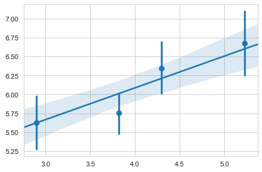
#x_bins把连续数据分割为离散数据
ax = sns.regplot(x=x, y=y, x_bins=4)

#非线性拟合：order设置拟合的项次（1表示线性，2,3,4...非线性）
ax = sns.regplot(x=x, y=y, order=2)

#转换成pandas Series数据格式
px = pd.Series(x, name='x_var')
py = pd.Series(y, name='y_var')
ax = sns.regplot(x=px, y=py, marker='+')

#logistic regression 逻辑回归
tips['big_tip'] = (tips.tip / tips.total_bill) > 0.175

ax = sns.regplot(x='total_bill', y='big_tip', data=tips,
                 logistic=True, n_boot=500, y_jitter=0.03)

#对数回归log
ax = sns.regplot(x='size', y='total_bill', data=tips,
                 x_estimator=np.mean, logx=True)

lmplot()

与regplot()功能相似，但结合regplot() 与 FacetGrid 功能。

sns.lmplot(
    x,
    y,
    data,
    hue=None,
    col=None,
    row=None,
    palette=None,
    col_wrap=None,
    height=5,
    aspect=1,
    markers='o',
    sharex=True,
    sharey=True,
    hue_order=None,
    col_order=None,
    row_order=None,
    legend=True,
    legend_out=True,
    x_estimator=None,
    x_bins=None,
    x_ci='ci',
    scatter=True,
    fit_reg=True,
    ci=95,
    n_boot=1000,
    units=None,
    order=1,
    logistic=False,
    lowess=False,
    robust=False,
    logx=False,
    x_partial=None,
    y_partial=None,
    truncate=False,
    x_jitter=None,
    y_jitter=None,
    scatter_kws=None,
    line_kws=None,
    size=None,
)
Docstring:
Plot data and regression model fits across a FacetGrid.

This function combines :func:`regplot` and :class:`FacetGrid`. It is
intended as a convenient interface to fit regression models across
conditional subsets of a dataset.

When thinking about how to assign variables to different facets, a general
rule is that it makes sense to use ``hue`` for the most important
comparison, followed by ``col`` and ``row``. However, always think about
your particular dataset and the goals of the visualization you are
creating.

There are a number of mutually exclusive options for estimating the
regression model. See the :ref:`tutorial <regression_tutorial>` for more
information.    

The parameters to this function span most of the options in
:class:`FacetGrid`, although there may be occasional cases where you will
want to use that class and :func:`regplot` directly.

Parameters
----------
x, y : strings, optional
    Input variables; these should be column names in ``data``.
data : DataFrame
    Tidy ("long-form") dataframe where each column is a variable and each
    row is an observation.
hue, col, row : strings
    Variables that define subsets of the data, which will be drawn on
    separate facets in the grid. See the ``*_order`` parameters to control
    the order of levels of this variable.
palette : palette name, list, or dict, optional
    Colors to use for the different levels of the ``hue`` variable. Should
    be something that can be interpreted by :func:`color_palette`, or a
    dictionary mapping hue levels to matplotlib colors.
col_wrap : int, optional
    "Wrap" the column variable at this width, so that the column facets
    span multiple rows. Incompatible with a ``row`` facet.
height : scalar, optional
    Height (in inches) of each facet. See also: ``aspect``.
aspect : scalar, optional
    Aspect ratio of each facet, so that ``aspect * height`` gives the width
    of each facet in inches.
markers : matplotlib marker code or list of marker codes, optional
    Markers for the scatterplot. If a list, each marker in the list will be
    used for each level of the ``hue`` variable.
share{x,y} : bool, 'col', or 'row' optional
    If true, the facets will share y axes across columns and/or x axes
    across rows.
{hue,col,row}_order : lists, optional
    Order for the levels of the faceting variables. By default, this will
    be the order that the levels appear in ``data`` or, if the variables
    are pandas categoricals, the category order.
legend : bool, optional
    If ``True`` and there is a ``hue`` variable, add a legend.
legend_out : bool, optional
    If ``True``, the figure size will be extended, and the legend will be
    drawn outside the plot on the center right.
x_estimator : callable that maps vector -> scalar, optional
    Apply this function to each unique value of ``x`` and plot the
    resulting estimate. This is useful when ``x`` is a discrete variable.
    If ``x_ci`` is given, this estimate will be bootstrapped and a
    confidence interval will be drawn.
x_bins : int or vector, optional
    Bin the ``x`` variable into discrete bins and then estimate the central
    tendency and a confidence interval. This binning only influences how
    the scatterplot is drawn; the regression is still fit to the original
    data.  This parameter is interpreted either as the number of
    evenly-sized (not necessary spaced) bins or the positions of the bin
    centers. When this parameter is used, it implies that the default of
    ``x_estimator`` is ``numpy.mean``.
x_ci : "ci", "sd", int in [0, 100] or None, optional
    Size of the confidence interval used when plotting a central tendency
    for discrete values of ``x``. If ``"ci"``, defer to the value of the
    ``ci`` parameter. If ``"sd"``, skip bootstrapping and show the
    standard deviation of the observations in each bin.
scatter : bool, optional
    If ``True``, draw a scatterplot with the underlying observations (or
    the ``x_estimator`` values).
fit_reg : bool, optional
    If ``True``, estimate and plot a regression model relating the ``x``
    and ``y`` variables.
ci : int in [0, 100] or None, optional
    Size of the confidence interval for the regression estimate. This will
    be drawn using translucent bands around the regression line. The
    confidence interval is estimated using a bootstrap; for large
    datasets, it may be advisable to avoid that computation by setting
    this parameter to None.
n_boot : int, optional
    Number of bootstrap resamples used to estimate the ``ci``. The default
    value attempts to balance time and stability; you may want to increase
    this value for "final" versions of plots.
units : variable name in ``data``, optional
    If the ``x`` and ``y`` observations are nested within sampling units,
    those can be specified here. This will be taken into account when
    computing the confidence intervals by performing a multilevel bootstrap
    that resamples both units and observations (within unit). This does not
    otherwise influence how the regression is estimated or drawn.
order : int, optional
    If ``order`` is greater than 1, use ``numpy.polyfit`` to estimate a
    polynomial regression.
logistic : bool, optional
    If ``True``, assume that ``y`` is a binary variable and use
    ``statsmodels`` to estimate a logistic regression model. Note that this
    is substantially more computationally intensive than linear regression,
    so you may wish to decrease the number of bootstrap resamples
    (``n_boot``) or set ``ci`` to None.
lowess : bool, optional
    If ``True``, use ``statsmodels`` to estimate a nonparametric lowess
    model (locally weighted linear regression). Note that confidence
    intervals cannot currently be drawn for this kind of model.
robust : bool, optional
    If ``True``, use ``statsmodels`` to estimate a robust regression. This
    will de-weight outliers. Note that this is substantially more
    computationally intensive than standard linear regression, so you may
    wish to decrease the number of bootstrap resamples (``n_boot``) or set
    ``ci`` to None.
logx : bool, optional
    If ``True``, estimate a linear regression of the form y ~ log(x), but
    plot the scatterplot and regression model in the input space. Note that
    ``x`` must be positive for this to work.
{x,y}_partial : strings in ``data`` or matrices
    Confounding variables to regress out of the ``x`` or ``y`` variables
    before plotting.
truncate : bool, optional
    By default, the regression line is drawn to fill the x axis limits
    after the scatterplot is drawn. If ``truncate`` is ``True``, it will
    instead by bounded by the data limits.
{x,y}_jitter : floats, optional
    Add uniform random noise of this size to either the ``x`` or ``y``
    variables. The noise is added to a copy of the data after fitting the
    regression, and only influences the look of the scatterplot. This can
    be helpful when plotting variables that take discrete values.
{scatter,line}_kws : dictionaries
    Additional keyword arguments to pass to ``plt.scatter`` and
    ``plt.plot``.    

See Also
--------
regplot : Plot data and a conditional model fit.
FacetGrid : Subplot grid for plotting conditional relationships.
pairplot : Combine :func:`regplot` and :class:`PairGrid` (when used with
           ``kind="reg"``).

#回归图
ax = sns.lmplot(x='total_bill', y='tip', data=tips)

#hue添加分类, markers设置散点样式
ax = sns.lmplot(x='total_bill', y='tip',
                hue="smoker", data=tips,
                markers=['o','x']
               )

#palette设置调色板
ax = sns.lmplot(x='total_bill', y='tip',
                hue='smoker', data=tips,
                palette='Set1'
               )

#palette设置调色板
ax = sns.lmplot(x='total_bill', y='tip',
                hue='smoker', data=tips,
                palette=dict(Yes='g', No='m')
               )

#col设置分栏绘制
ax = sns.lmplot(x='total_bill', y='tip',
                col='smoker', data=tips
               )

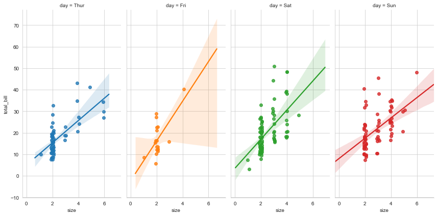
#heigtht图高，aspect宽/高比例,x_jitter添加数据噪点
ax = sns.lmplot(x='size', y='total_bill', hue='day',
                col='day', data=tips,
                height=6, aspect=0.5,
                x_jitter=.1
               )

#col_wrap设置多行显示
ax = sns.lmplot(x='total_bill', y='tip', hue='day',
                col='day', data=tips,
                col_wrap=2, height=3
               )

#多行多栏显示
ax = sns.lmplot(x='total_bill', y='tip',
                row='sex', col='time',
                data=tips, height=3
               )

ax = sns.lmplot(x='total_bill', y='tip',
                row='sex', col='time',
                data=tips, height=3
               )

#设置图形参数
ax = ax.set_axis_labels("Total bill (US Dollars)", "Tip")
ax = ax.set(xlim=(0,60), ylim=(0,12),
            xticks=[10, 30, 50], yticks=[2, 6, 10])
ax = ax.fig.subplots_adjust(wspace=.02)