《DSP using MATLAB》Problem 8.32

代码：

%% ------------------------------------------------------------------------
%%            Output Info about this m-file
fprintf('\n***********************************************************\n');
fprintf('        <DSP using MATLAB> Problem 8.32 \n\n');

banner();
%% ------------------------------------------------------------------------

% -------------------------------------
%           Ω=(2/T)tan(ω/2)
%           ω=2*[atan(ΩT/2)]
%     Digital Filter Specifications:
% -------------------------------------
wp = 0.3*pi;                     % digital passband freq in rad
ws = 0.4*pi;                     % digital stopband freq in rad
Rp = 0.25;                       % passband ripple in dB
As = 50;                         % stopband attenuation in dB

Ripple = 10 ^ (-Rp/20)           % passband ripple in absolute
Attn = 10 ^ (-As/20)             % stopband attenuation in absolute

% Analog prototype specifications: Inverse Mapping for frequencies
T = 1;                           % set T = 1
Fs = 1/T;
OmegaP = (2/T)*tan(wp/2)        % prototype passband freq
OmegaS = (2/T)*tan(ws/2)        % prototype stopband freq      

% Analog Elliptic Prototype Filter Calculation:
[cs, ds] = afd_elip(OmegaP, OmegaS, Rp, As);

% Calculation of second-order sections:
fprintf('\n***** Cascade-form in s-plane: START *****\n');
[CS, BS, AS] = sdir2cas(cs, ds)
fprintf('\n***** Cascade-form in s-plane: END *****\n');

% Calculation of Frequency Response:
[db_s, mag_s, pha_s, ww_s] = freqs_m(cs, ds, 0.5*pi/T);

% Calculation of Impulse Response:
[ha, x, t] = impulse(cs, ds);

% Impulse Invariance Transformation:
%[b, a] = imp_invr(cs, ds, T); 

% Bilinear Transformation
[b, a] = bilinear(cs, ds, Fs)
[C, B, A] = dir2cas(b, a)

% Calculation of Frequency Response:
[db, mag, pha, grd, ww] = freqz_m(b, a);

%% -----------------------------------------------------------------
%%                             Plot
%% -----------------------------------------------------------------
figure('NumberTitle', 'off', 'Name', 'Problem 8.32 Analog Elliptic lowpass')
set(gcf,'Color','white');
M = 1.0;                          % Omega max

subplot(2,2,1); plot(ww_s/pi, mag_s);  grid on; %axis([-10, 10, 0, 1.2]);
xlabel(' Analog frequency in \pi units'); ylabel('|H|'); title('Magnitude in Absolute');
set(gca, 'XTickMode', 'manual', 'XTick', [-0.4625, -0.3244, 0, 0.3244, 0.4625]);
set(gca, 'YTickMode', 'manual', 'YTick', [0, 0.0032, 0.9716, 1.0, 1.5]);

subplot(2,2,2); plot(ww_s/pi, db_s);  grid on; %axis([0, M, -50, 10]);
xlabel('Analog frequency in \pi units'); ylabel('Decibels'); title('Magnitude in dB ');
set(gca, 'XTickMode', 'manual', 'XTick', [-0.4625, -0.3244, 0, 0.3244, 0.417, 0.458, 0.4625]);
set(gca, 'YTickMode', 'manual', 'YTick', [-50, -1, 0]);
set(gca,'YTickLabelMode','manual','YTickLabel',['50';' 1';' 0']);

subplot(2,2,3); plot(ww_s/pi, pha_s/pi);  grid on; %axis([-10, 10, -1.2, 1.2]);
xlabel('Analog frequency in \pi nuits'); ylabel('radians'); title('Phase Response');
set(gca, 'XTickMode', 'manual', 'XTick', [-0.4625, -0.3244, 0, 0.3244, 0.4625]);
set(gca, 'YTickMode', 'manual', 'YTick', [-1:0.5:1]);

subplot(2,2,4); plot(t, ha); grid on; %axis([0, 30, -0.05, 0.25]);
xlabel('time in seconds'); ylabel('ha(t)'); title('Impulse Response');

figure('NumberTitle', 'off', 'Name', 'Problem 8.32 Digital Elliptic lowpass by bilinear')
set(gcf,'Color','white');
M = 2;                          % Omega max

subplot(2,2,1); plot(ww/pi, mag); axis([0, M, 0, 1.2]); grid on;
xlabel(' Digital frequency in \pi units'); ylabel('|H|'); title('Magnitude Response');
set(gca, 'XTickMode', 'manual', 'XTick', [0, 0.3, 0.4, 1.6, 1.7, M]);
set(gca, 'YTickMode', 'manual', 'YTick', [0, 0.0032, 0.9716, 1]);

subplot(2,2,2); plot(ww/pi, pha/pi); axis([0, M, -1.1, 1.1]); grid on;
xlabel('Digital frequency in \pi nuits'); ylabel('radians in \pi units'); title('Phase Response');
set(gca, 'XTickMode', 'manual', 'XTick', [0, 0.3, 0.4, 1.6, 1.7, M]);
set(gca, 'YTickMode', 'manual', 'YTick', [-1:1:1]);

subplot(2,2,3); plot(ww/pi, db); axis([0, M, -80, 10]); grid on;
xlabel('Digital frequency in \pi units'); ylabel('Decibels'); title('Magnitude in dB ');
set(gca, 'XTickMode', 'manual', 'XTick', [0, 0.3, 0.37, 0.4, 1.6, 1.7, M]);
set(gca, 'YTickMode', 'manual', 'YTick', [-60, -50, -1, 0]);
set(gca,'YTickLabelMode','manual','YTickLabel',['60';'50';' 1';' 0']);

subplot(2,2,4); plot(ww/pi, grd); grid on; %axis([0, M, 0, 35]);
xlabel('Digital frequency in \pi units'); ylabel('Samples'); title('Group Delay');
set(gca, 'XTickMode', 'manual', 'XTick', [0, 0.3, 0.4, 1.6, 1.7, M]);
%set(gca, 'YTickMode', 'manual', 'YTick', [0:5:35]);

figure('NumberTitle', 'off', 'Name', 'Problem 8.32 Pole-Zero Plot')
set(gcf,'Color','white');
zplane(b,a);
title(sprintf('Pole-Zero Plot'));
%pzplotz(b,a);

% ----------------------------------------------
%       Calculation of Impulse Response
% ----------------------------------------------
figure('NumberTitle', 'off', 'Name', 'Problem 8.32 Imp & Freq Response')
set(gcf,'Color','white');
t = [0:0.01:90]; subplot(2,1,1); impulse(cs,ds,t); grid on;   % Impulse response of the analog filter
axis([0,90,-0.2,0.3]);hold on

n = [0:1:90/T]; hn = filter(b,a,impseq(0,0,90/T));           % Impulse response of the digital filter
stem(n*T,hn); xlabel('time in sec'); title (sprintf('Impulse Responses T=%2d',T));
hold off

% Calculation of Frequency Response:
[dbs, mags, phas, wws] = freqs_m(cs, ds, 2*pi/T);             % Analog frequency   s-domain  

[dbz, magz, phaz, grdz, wwz] = freqz_m(b, a);                  % Digital  z-domain

%% -----------------------------------------------------------------
%%                             Plot
%% -----------------------------------------------------------------  

subplot(2,1,2); plot(wws/(2*pi), mags/T,'b', wwz/(2*pi*T), magz, 'r'); grid on;

xlabel('frequency in Hz'); title('Magnitude Responses'); ylabel('Magnitude'); 

text(-0.8,0.15,'Analog filter', 'Color', 'b'); text(0.8,0.4,'Digital filter', 'Color', 'r');

　　运行结果：

这里主要放双线性变化法的代码。

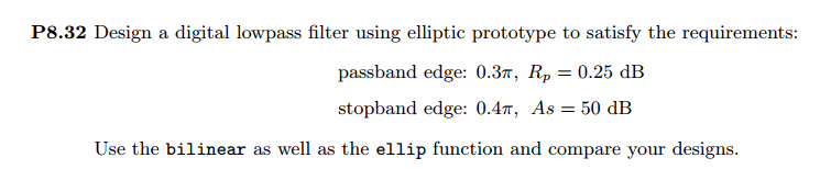
通带、阻带绝对指标，模拟滤波器截止频率指标，

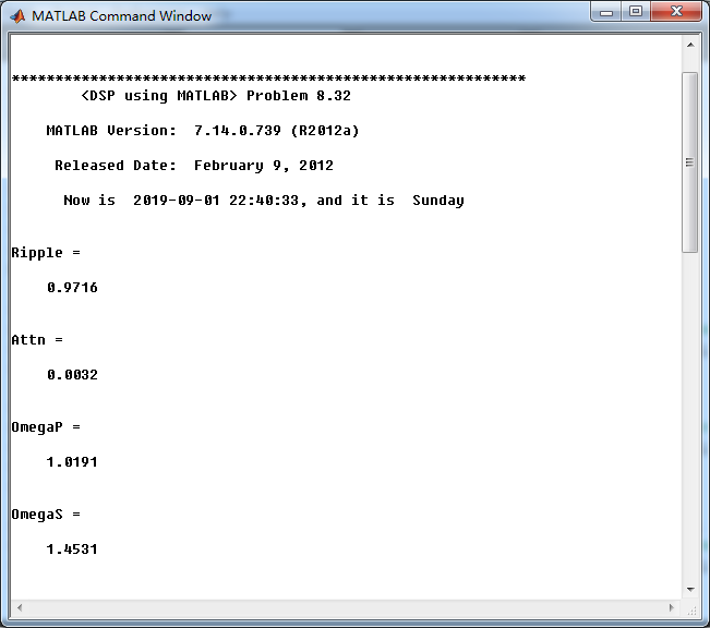
模拟Elliptic原型低通滤波器，系统函数串联形式的系数

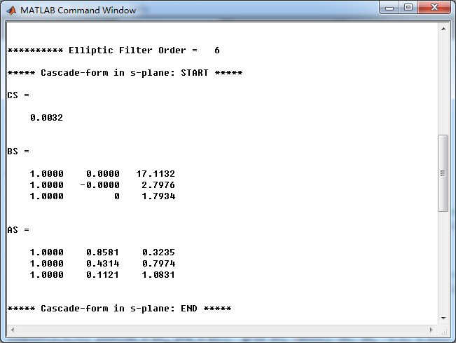
采用双线性变换法，得到数字Elliptic低通滤波器，系统函数直接形式的系数，转换成串联形式的系数

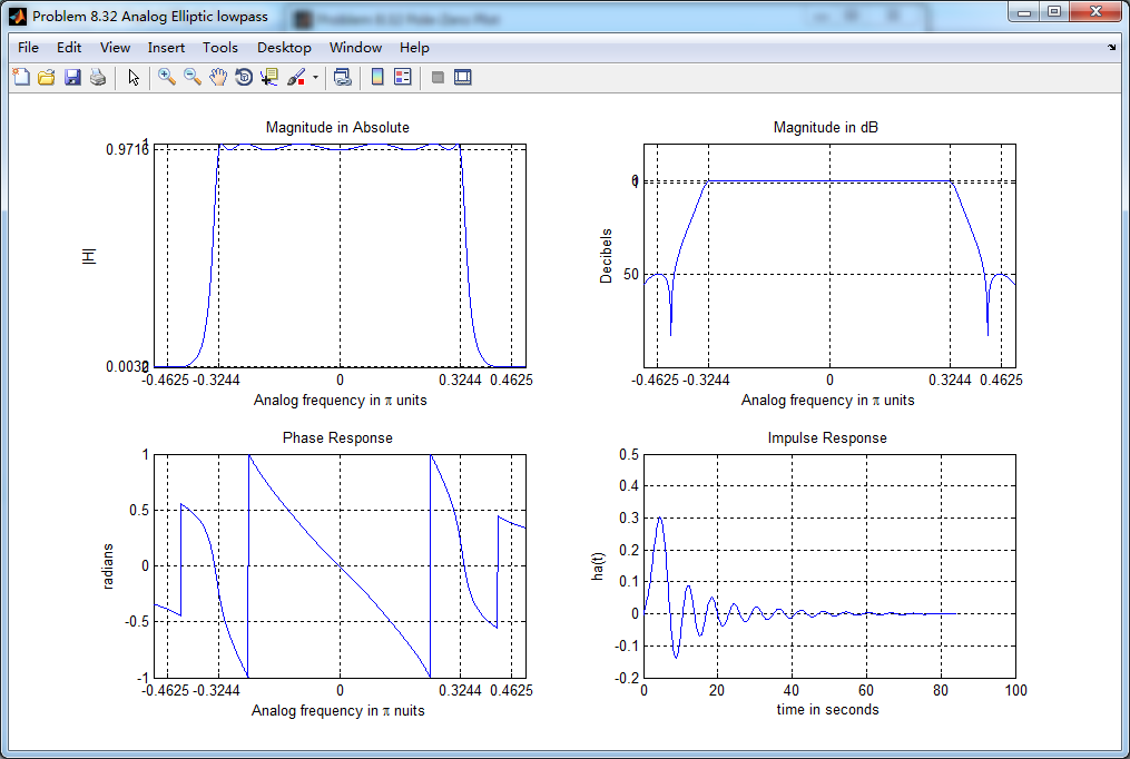
模拟Elliptic原型低通滤波器，其幅度谱、相位谱和脉冲响应

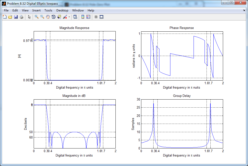
采用双线性变换法（bilinear）得到数字Elliptic低通滤波器，其幅度谱、相位谱和群延迟响应

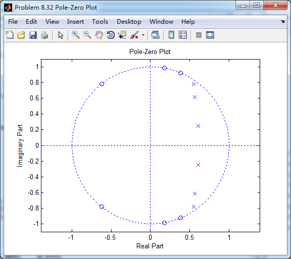
数字Elliptic低通系统函数零极点图

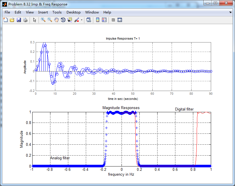
模拟原型和数字低通的脉冲响应对比，可见双线性变换法不保留脉冲响应的形态。

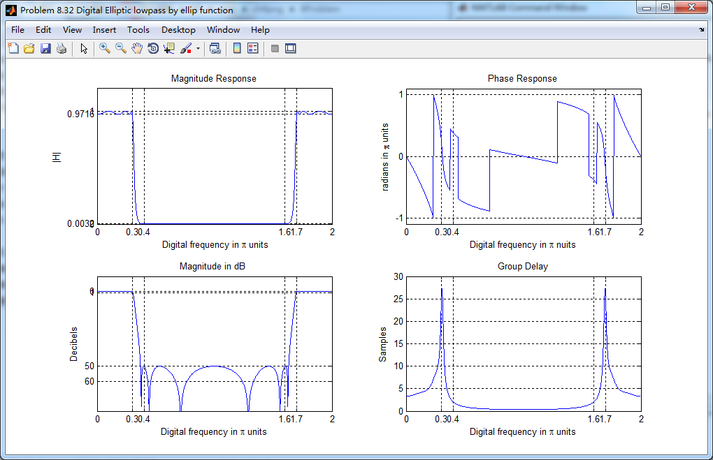
使用MATLAB自带ellip函数的运算结果这里就不写了，只放张幅度谱、相位谱和群延迟响应的图，可见和双线性变换法得到的结果相比，区别不大。