吴裕雄--天生自然 R语言开发学习：方差分析

#-------------------------------------------------------------------#
# R in Action (2nd ed): Chapter 9                                   #
# Analysis of variance                                              #
# requires packages multcomp, gplots, car, HH, effects,             #
#                   rrcov, mvoutlier to be installed                #
# install.packages(c("multcomp", "gplots", "car", "HH", "effects",  #
#                    "rrcov", "mvoutlier"))                         #
#-------------------------------------------------------------------#

par(ask=TRUE)
opar <- par(no.readonly=TRUE) # save original parameters

# Listing 9.1 - One-way ANOVA
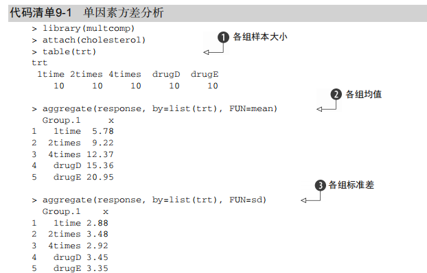
library(multcomp)
attach(cholesterol)
table(trt)
aggregate(response, by=list(trt), FUN=mean)
aggregate(response, by=list(trt), FUN=sd)
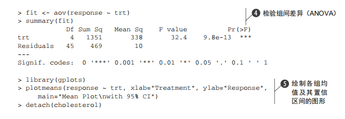
fit <- aov(response ~ trt)
summary(fit)
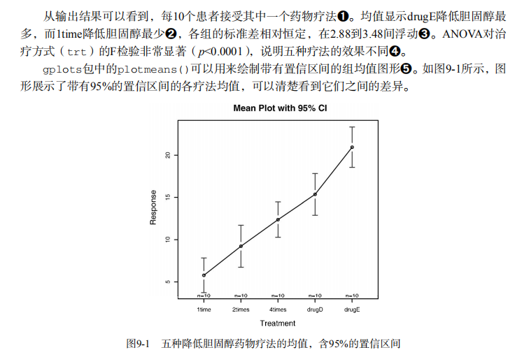
library(gplots)
plotmeans(response ~ trt, xlab="Treatment", ylab="Response",
          main="Mean Plot\nwith 95% CI")
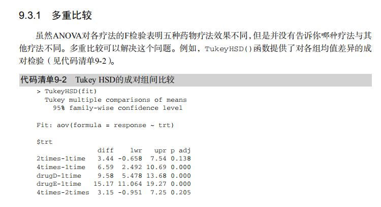
detach(cholesterol)

# Listing 9.2 - Tukey HSD pairwise group comparisons
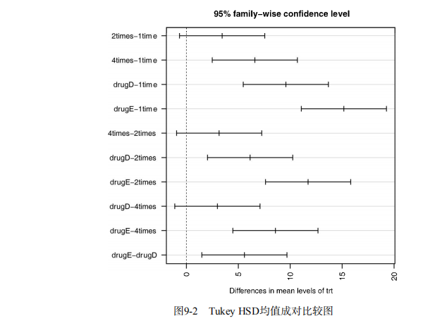
TukeyHSD(fit)
par(las=2)
par(mar=c(5,8,4,2))
plot(TukeyHSD(fit))
par(opar)

# Multiple comparisons the multcomp package
library(multcomp)
par(mar=c(5,4,6,2))
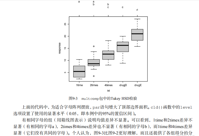
tuk <- glht(fit, linfct=mcp(trt="Tukey"))
plot(cld(tuk, level=.05),col="lightgrey")
par(opar)

# Assessing normality
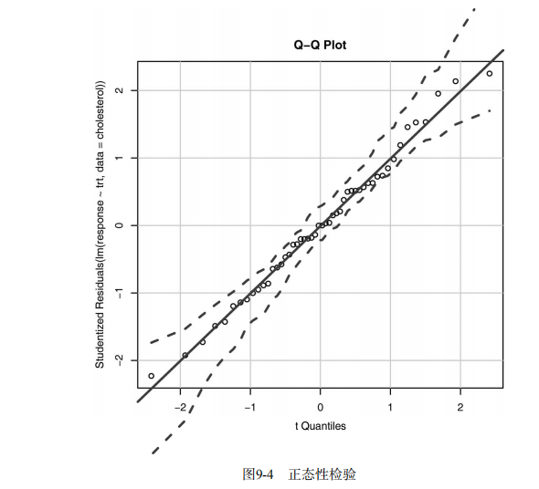
library(car)
qqPlot(lm(response ~ trt, data=cholesterol),
       simulate=TRUE, main="Q-Q Plot", labels=FALSE)

# Assessing homogeneity of variances
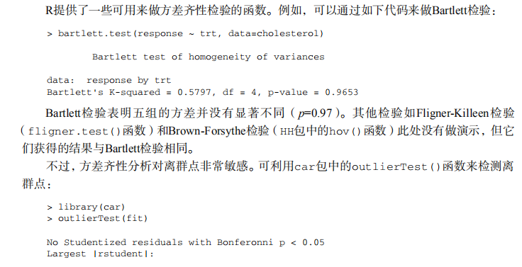
bartlett.test(response ~ trt, data=cholesterol)

# Assessing outliers
library(car)
outlierTest(fit)

# Listing 9.3 - One-way ANCOVA
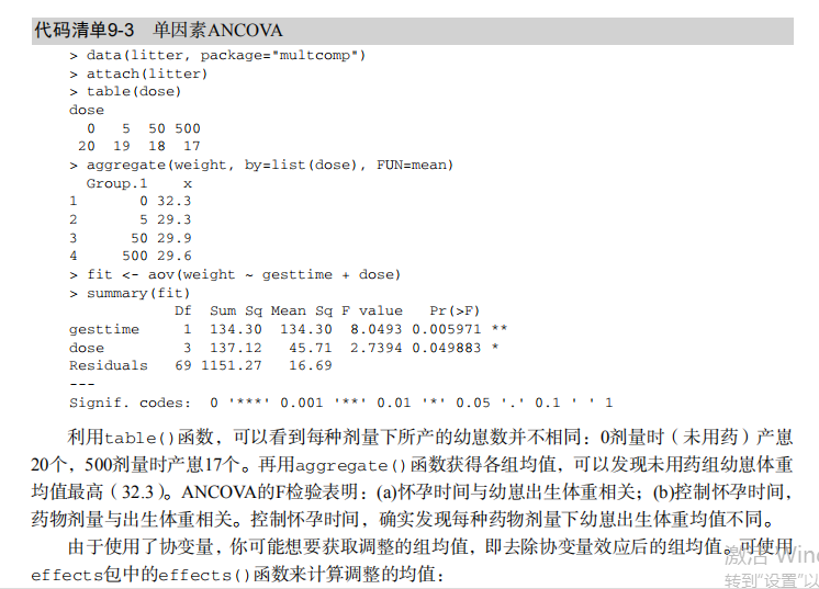
data(litter, package="multcomp")
attach(litter)
table(dose)
aggregate(weight, by=list(dose), FUN=mean)
fit <- aov(weight ~ gesttime + dose)
summary(fit)

# Obtaining adjusted means
library(effects)
effect("dose", fit)

#  Listing 9.4 - Multiple comparisons using user supplied contrasts
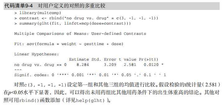
library(multcomp)
contrast <- rbind("no drug vs. drug" = c(3, -1, -1, -1))
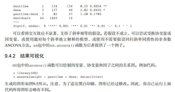
summary(glht(fit, linfct=mcp(dose=contrast)))

# Listing 9.5 - Testing for homegeneity of regression slopes
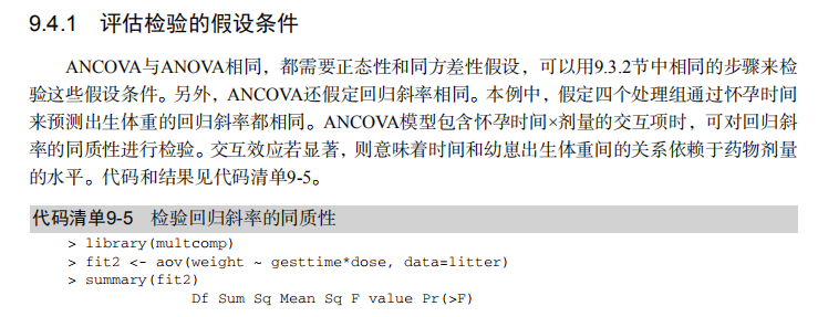
library(multcomp)
fit2 <- aov(weight ~ gesttime*dose, data=litter)
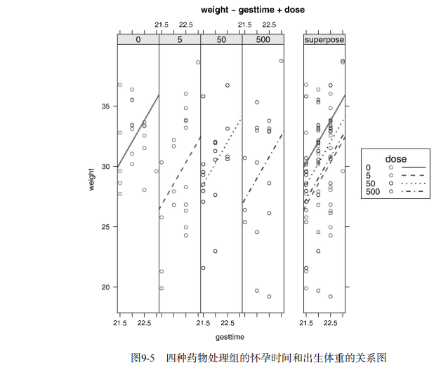
summary(fit2)

# Visualizing a one-way ANCOVA
library(HH)
ancova(weight ~ gesttime + dose, data=litter)

# Listing 9.6 - Two way ANOVA
attach(ToothGrowth)
table(supp,dose)
aggregate(len, by=list(supp,dose), FUN=mean)
aggregate(len, by=list(supp,dose), FUN=sd)
dose <- factor(dose)
fit <- aov(len ~ supp*dose)
summary(fit)

# plotting interactions
interaction.plot(dose, supp, len, type="b",
                 col=c("red","blue"), pch=c(16, 18),
                 main = "Interaction between Dose and Supplement Type")
library(gplots)
plotmeans(len ~ interaction(supp, dose, sep=" "),
          connect=list(c(1, 3, 5),c(2, 4, 6)),
          col=c("red","darkgreen"),
          main = "Interaction Plot with 95% CIs",
          xlab="Treatment and Dose Combination")
library(HH)
interaction2wt(len~supp*dose)

#  Listing 9.7 - Repeated measures ANOVA with one between and within groups factor
CO2$conc <- factor(CO2$conc)
w1b1 <- subset(CO2, Treatment=='chilled')
fit <- aov(uptake ~ (conc*Type) + Error(Plant/(conc)), w1b1)
summary(fit)
par(las=2)
par(mar=c(10,4,4,2))
with(w1b1,
     interaction.plot(conc,Type,uptake,
                      type="b", col=c("red","blue"), pch=c(16,18),
                      main="Interaction Plot for Plant Type and Concentration"))
boxplot(uptake ~ Type*conc, data=w1b1, col=(c("gold","green")),
        main="Chilled Quebec and Mississippi Plants",
        ylab="Carbon dioxide uptake rate (umol/m^2 sec)")
par(opar)

# Listing 9.8 - One-way MANOVA
library(MASS)
attach(UScereal)
shelf <- factor(shelf)
y <- cbind(calories, fat, sugars)
aggregate(y, by=list(shelf), FUN=mean)
cov(y)
fit <- manova(y ~ shelf)
summary(fit)
summary.aov(fit)

#  Listing 9.9 - Assessing multivariate normality
center <- colMeans(y)
n <- nrow(y)
p <- ncol(y)
cov <- cov(y)
d <- mahalanobis(y,center,cov)
coord <- qqplot(qchisq(ppoints(n),df=p),
                d, main="QQ Plot Assessing Multivariate Normality",
                ylab="Mahalanobis D2")
abline(a=0,b=1)
identify(coord$x, coord$y, labels=row.names(UScereal))

# multivariate outliers
library(mvoutlier)
outliers <- aq.plot(y)
outliers

# Listing 9.10 - Robust one-way MANOVA
library(rrcov)
Wilks.test(y,shelf, method="mcd")  # this can take a while

# Listing 9.11 - A regression approach to the Anova problem
fit.lm <- lm(response ~ trt, data=cholesterol)
summary(fit.lm)
contrasts(cholesterol$trt)