ML(4)——逻辑回归
Logistic Regression虽然名字里带“回归”,但是它实际上是一种分类方法,“逻辑”是Logistic的音译,和真正的逻辑没有任何关系。
模型
线性模型
由于逻辑回归是一种分类方法,所以我们仍然以最简的二分类为例。与感知机不同,对于逻辑回归的分类结果,y ∈ {0, 1},我们需要找到最佳的hθ(x)拟合数据。
这里容易联想到线性回归。线性回归也可以用于分类,但是很多时候,尤其是二分类的时候,线性回归并不能很好地工作,因为分类不是连续的函数,其结果只能是固定的离散值。设想一下有线性回归得到的拟合曲线hθ(x),当x→∞时,有可能y→∞,这就无法对y ∈ {0, 1}进行有效解释。
对于二分类,逻辑回归的目的是找到一个函数,使得无论x取何值,都有:

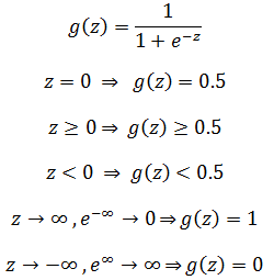
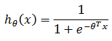
满足这个式子的典型函数是sigmoid函数,也称为logistic函数:
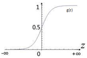
在sigmoid函数g(z)中:
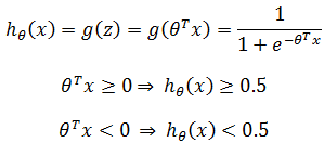
现在,将hθ(x)赋予sigmoid函数g(z)的特性:
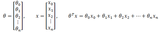
其中:
最终,逻辑回归的模型函数:

假设给定一些输入,现在需要根据逻辑回归模型预测肿瘤是否是良性,最终得到hθ(x) = 0.8,可以用概率表述:

上式表示在当前输入下,y=1的概率是0.8,y=0的概率是0.2,因为是分类,所以判断y = 1。
需要注意的是,sigmoid函数不是样本点的分隔曲线,它表示的是逻辑回归的测结果;θTx才是分隔曲线,它将样本点分为θTx ≥ 0和θTx < 0两部分:

分隔曲线

Sigmoid函数,最终模型
由此看来,逻辑回归的线性模型同样是找到最佳的θ,使两类样本点分离,这就在很大程度上和感知机相似。
多项式模型
直观地看,线性模型的决策边界就是将两类样本点分离开的分隔曲线,我们之前已经多次接触过,只是没有给它起一个专业的名字。假设在一个模型中,hθ(x) = g(θ0 + θ1x1 + θ2x2) = g(-3 + x1 + x2),那么决策边界就是 -3 + x1 + x2 = 0:

很多时候,直线并不能很好地作为决策边界,如下图所示:
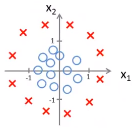
此时需要使用多项式模型添加更多的特征:
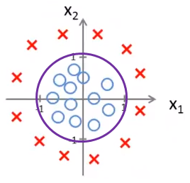

这相当于添加了两个新的特征:

深入了解不同函数的特征有助于选择正确的模型。添加的特征越多,曲线越复杂,对训练样本的拟合度越高,同时也更容易导致过拟合而丧失泛化性:

关于过拟合及其处理,可参考《ML(附录3)——数据拟合和正则化》。
多分类
我们已经知道了二分类的模型,然而实际问题中往往不只是二分类,那么逻辑回归如何处理多分类呢?
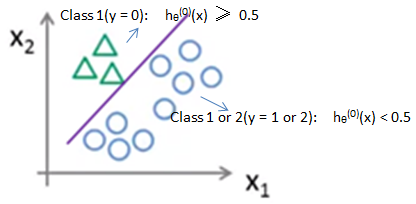
一种可行的方法就是化繁为简,将多分类转换为二分类:

如上图所示,三分类转换为三个二分类,其中上标表示分类的类别:
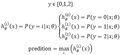
对于输入x,其预测结果是所有hθ(x)中值最大的一个。对于最后的预测结论,以上面的三分类为例,如果输入一个标签为2的特征集,对于hθ(0)(x) 来说,hθ(0)(x) < 0.5:
对于hθ(1)(x) 来说,hθ(1)(x) < 0.5:

对于hθ(3)(x) 来说,hθ(3)(x) ≥ 0.5:

因此,对于输入x,其预测结果是所有hθ(x)中值最大的一个。至于每个样本标签值是多少,无所谓了,在训练每个hθ(i)(x)前,都需要把y(i) 转换为1,其余转换为0。
在上面的图组中也可以看出,对于有k个标签的多分类,需要训练k个不同的逻辑回归模型。
学习策略
在感知机中,模型函数使用了sign,由于sign是阶跃函数,不易优化,所以为了求得损失函数,我们使用函数间隔进行了一系列转换。对于逻辑回归,由于函数本身是连续曲线,所以不会存在这样的问题,其J(θ)使用对数损失函数。对数损失函数的原型:

将其用在逻辑回归上:
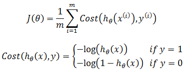
这里的对数是以e为底的对数,即:
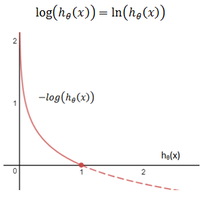
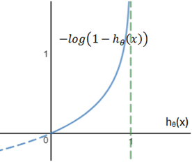
注意,0 < hθ(x) < 1。上图是y = 1时的costfunction,可以看到,当hθ(x)→1时,Cost(hθ(x), y)→0;当hθ(x)→0时,Cost(hθ(x),y)→∞。也就是说当分类是1时,sigmoid的值越接近于1,损失值越小;sigmoid的值越接近于0,损失值越大。损失值越大,分类点越接近决策面,其分类越模糊。与此类似,下图是 y = 0时的cost function:
Cost function可以把y = 1和y=1两种情况合并到一起:

理解这种形式需要再次将y分开:
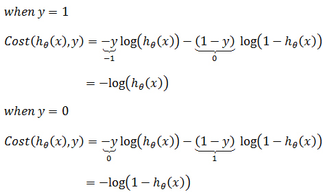
最后得到J(θ)的最终形式:
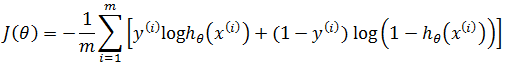
注意,这里hθ(x)是sigmoid函数:
如果写成矩阵的形式:
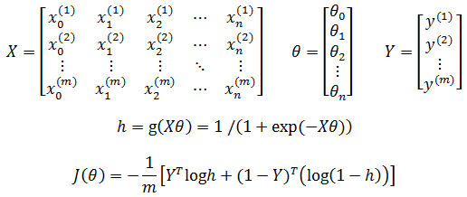
上式中,hθ(x)的操作对应矩阵中的每个元素,1-Y,log hθ(x)也一样,可参照后文的代码实现来理解。
算法
与之前的算法一样,我们的目的是找到最佳的θ使得J(θ)最小化,将求解θ转换为最优化问题,即:

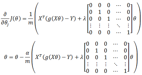
梯度下降
梯度下降是一个适用范围很广的方法,这里同样可以使用梯度下降求解θ:

关于梯度下降的更多内容可参考《ML(附录1)——梯度下降》。
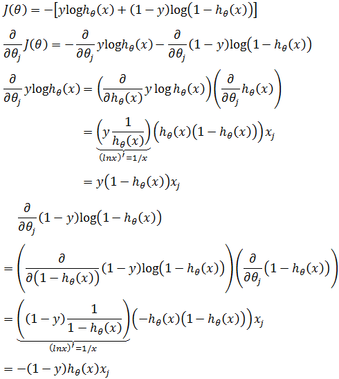
在对J(θ)求偏导时先做一些准备工作,计算sigmoid函数的导数(关于偏导和一元函数的导数,可参考《多变量微积分》和《单变量微积分》的相关章节):
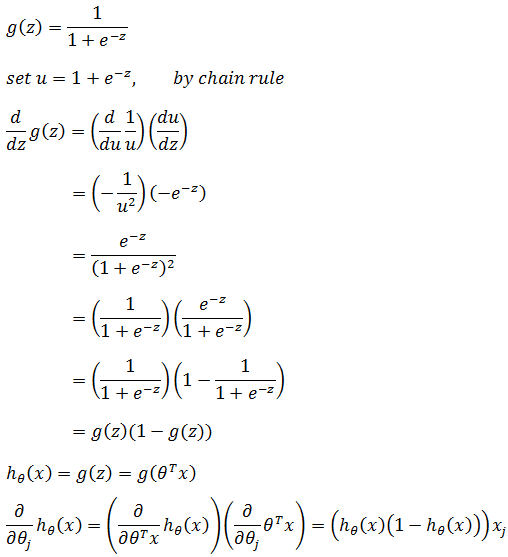
现在计算m=1时J(θ)的偏导,此时可以删除上标:

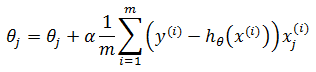
推广到m个样本:

在《机器学习实战》中提到对极大似然数使用梯度上升求最大值,最后得到:
这和对损失函数采用梯度下降求最小值是一样的,因为损失函数使用了似然数的负数形式,Cost(X, Y) = -logP(Y|X),所以对-logP(Y|X)梯度下降和对+logP(Y|X)梯度上升将得到同样的结果。
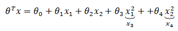
对于多项式模型,需要预先添加特征,使得每个θj都有唯一的xj对应:
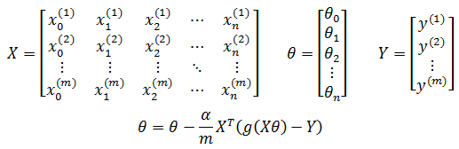
如果用矩阵表示:
在此基础上使用L2正则化(关于正则化,可参考《ML(附录3)——过拟合与欠拟合》):
代码实现
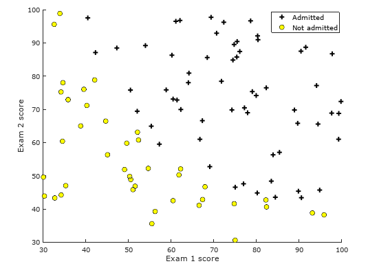
ex2data1.txt:
 34.62365962451697,78.0246928153624,

 30.28671076822607,43.89499752400101,

 35.84740876993872,72.90219802708364,

 60.18259938620976,86.30855209546826,

 79.0327360507101,75.3443764369103,

 45.08327747668339,56.3163717815305,

 61.10666453684766,96.51142588489624,

 75.02474556738889,46.55401354116538,

 76.09878670226257,87.42056971926803,

 84.43281996120035,43.53339331072109,

 95.86155507093572,38.22527805795094,

 75.01365838958247,30.60326323428011,

 82.30705337399482,76.48196330235604,

 69.36458875970939,97.71869196188608,

 39.53833914367223,76.03681085115882,

 53.9710521485623,89.20735013750205,

 69.07014406283025,52.74046973016765,

 67.94685547711617,46.67857410673128,

 70.66150955499435,92.92713789364831,

 76.97878372747498,47.57596364975532,

 67.37202754570876,42.83843832029179,

 89.67677575072079,65.79936592745237,

 50.534788289883,48.85581152764205,

 34.21206097786789,44.20952859866288,

 77.9240914545704,68.9723599933059,

 62.27101367004632,69.95445795447587,

 80.1901807509566,44.82162893218353,

 93.114388797442,38.80067033713209,

 61.83020602312595,50.25610789244621,

 38.78580379679423,64.99568095539578,

 61.379289447425,72.80788731317097,

 85.40451939411645,57.05198397627122,

 52.10797973193984,63.12762376881715,

 52.04540476831827,69.43286012045222,

 40.23689373545111,71.16774802184875,

 54.63510555424817,52.21388588061123,

 33.91550010906887,98.86943574220611,

 64.17698887494485,80.90806058670817,

 74.78925295941542,41.57341522824434,

 34.1836400264419,75.2377203360134,

 83.90239366249155,56.30804621605327,

 51.54772026906181,46.85629026349976,

 94.44336776917852,65.56892160559052,

 82.36875375713919,40.61825515970618,

 51.04775177128865,45.82270145776001,

 62.22267576120188,52.06099194836679,

 77.19303492601364,70.45820000180959,

 97.77159928000232,86.7278223300282,

 62.07306379667647,96.76882412413983,

 91.56497449807442,88.69629254546599,

 79.94481794066932,74.16311935043758,

 99.2725269292572,60.99903099844988,

 90.54671411399852,43.39060180650027,

 34.52451385320009,60.39634245837173,

 50.2864961189907,49.80453881323059,

 49.58667721632031,59.80895099453265,

 97.64563396007767,68.86157272420604,

 32.57720016809309,95.59854761387875,

 74.24869136721598,69.82457122657193,

 71.79646205863379,78.45356224515052,

 75.3956114656803,85.75993667331619,

 35.28611281526193,47.02051394723416,

 56.25381749711624,39.26147251058019,

 30.05882244669796,49.59297386723685,

 44.66826172480893,66.45008614558913,

 66.56089447242954,41.09209807936973,

 40.45755098375164,97.53518548909936,

 49.07256321908844,51.88321182073966,

 80.27957401466998,92.11606081344084,

 66.74671856944039,60.99139402740988,

 32.72283304060323,43.30717306430063,

 64.0393204150601,78.03168802018232,

 72.34649422579923,96.22759296761404,

 60.45788573918959,73.09499809758037,

 58.84095621726802,75.85844831279042,

 99.82785779692128,72.36925193383885,

 47.26426910848174,88.47586499559782,

 50.45815980285988,75.80985952982456,

 60.45555629271532,42.50840943572217,

 82.22666157785568,42.71987853716458,

 88.9138964166533,69.80378889835472,

 94.83450672430196,45.69430680250754,

 67.31925746917527,66.58935317747915,

 57.23870631569862,59.51428198012956,

 80.36675600171273,90.96014789746954,

 68.46852178591112,85.59430710452014,

 42.0754545384731,78.84478600148043,

 75.47770200533905,90.42453899753964,

 78.63542434898018,96.64742716885644,

 52.34800398794107,60.76950525602592,

 94.09433112516793,77.15910509073893,

 90.44855097096364,87.50879176484702,

 55.48216114069585,35.57070347228866,

 74.49269241843041,84.84513684930135,

 89.84580670720979,45.35828361091658,

 83.48916274498238,48.38028579728175,

 42.2617008099817,87.10385094025457,

 99.31500880510394,68.77540947206617,

 55.34001756003703,64.9319380069486,

 74.77589300092767,89.52981289513276,
Octave
%% Machine Learning Online Class - Exercise 2: Logistic Regression
%
% Instructions
% ------------
%
% This file contains code that helps you get started on the logistic
% regression exercise. You will need to complete the following functions
% in this exericse:
%
% sigmoid.m
% costFunction.m
% predict.m
% costFunctionReg.m
%
% For this exercise, you will not need to change any code in this file,
% or any other files other than those mentioned above.
% %% Initialization
clear ; close all; clc %% Load Data
% The first two columns contains the exam scores and the third column
% contains the label. data = load('ex2data1.txt');
X = data(:, [1, 2]); y = data(:, 3); %% ==================== Part 1: Plotting ====================
% We start the exercise by first plotting the data to understand the
% the problem we are working with. fprintf(['Plotting data with + indicating (y = 1) examples and o ' ...
'indicating (y = 0) examples.\n']); plotData(X, y); % Put some labels
hold on;
% Labels and Legend
xlabel('Exam 1 score')
ylabel('Exam 2 score') % Specified in plot order
legend('Admitted', 'Not admitted')
hold off; fprintf('\nProgram paused. Press enter to continue.\n');
pause; %% ============ Part 2: Compute Cost and Gradient ============
% In this part of the exercise, you will implement the cost and gradient
% for logistic regression. You neeed to complete the code in
% costFunction.m % Setup the data matrix appropriately, and add ones for the intercept term
[m, n] = size(X); % Add intercept term to x and X_test
X = [ones(m, 1) X]; % Initialize fitting parameters
initial_theta = zeros(n + 1, 1); % Compute and display initial cost and gradient
[cost, grad] = costFunction(initial_theta, X, y); fprintf('Cost at initial theta (zeros): %f\n', cost);
fprintf('Expected cost (approx): 0.693\n');
fprintf('Gradient at initial theta (zeros): \n');
fprintf(' %f \n', grad);
fprintf('Expected gradients (approx):\n -0.1000\n -12.0092\n -11.2628\n'); % Compute and display cost and gradient with non-zero theta
test_theta = [-24; 0.2; 0.2];
[cost, grad] = costFunction(test_theta, X, y); fprintf('\nCost at test theta: %f\n', cost);
fprintf('Expected cost (approx): 0.218\n');
fprintf('Gradient at test theta: \n');
fprintf(' %f \n', grad);
fprintf('Expected gradients (approx):\n 0.043\n 2.566\n 2.647\n'); fprintf('\nProgram paused. Press enter to continue.\n');
pause; %% ============= Part 3: Optimizing using fminunc =============
% In this exercise, you will use a built-in function (fminunc) to find the
% optimal parameters theta. % Set options for fminunc
options = optimset('GradObj', 'on', 'MaxIter', 400);
% Run fminunc to obtain the optimal theta
% This function will return theta and the cost
[theta, cost] = fminunc(@(t)(costFunction(t, X, y)), initial_theta, options);
% Print theta to screen
fprintf('Cost at theta found by fminunc: %f\n', cost);
fprintf('Expected cost (approx): 0.203\n');
fprintf('theta: \n');
fprintf(' %f \n', theta);
fprintf('Expected theta (approx):\n');
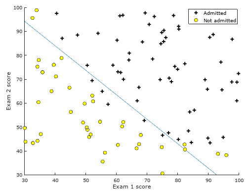
fprintf(' -25.161\n 0.206\n 0.201\n'); % Plot Boundary
plotDecisionBoundary(theta, X, y); % Put some labels
hold on;
% Labels and Legend
xlabel('Exam 1 score')
ylabel('Exam 2 score') % Specified in plot order
legend('Admitted', 'Not admitted')
hold off; fprintf('\nProgram paused. Press enter to continue.\n');
pause; %% ============== Part 4: Predict and Accuracies ==============
% After learning the parameters, you'll like to use it to predict the outcomes
% on unseen data. In this part, you will use the logistic regression model
% to predict the probability that a student with score 45 on exam 1 and
% score 85 on exam 2 will be admitted.
%
% Furthermore, you will compute the training and test set accuracies of
% our model.
%
% Your task is to complete the code in predict.m % Predict probability for a student with score 45 on exam 1
% and score 85 on exam 2 prob = sigmoid([1 45 85] * theta);
fprintf(['For a student with scores 45 and 85, we predict an admission ' ...
'probability of %f\n'], prob);
fprintf('Expected value: 0.775 +/- 0.002\n\n'); % Compute accuracy on our training set
p = predict(theta, X); fprintf('Train Accuracy: %f\n', mean(double(p == y)) * 100);
fprintf('Expected accuracy (approx): 89.0\n');
fprintf('\n');
plotData.m
function plotData(X, y)

%PLOTDATA Plots the data points X and y into a new figure

%   PLOTDATA(x,y) plots the data points with + for the positive examples

%   and o for the negative examples. X is assumed to be a Mx2 matrix.

% Create New Figure

  figure; hold on;

% Instructions: Plot the positive and negative examples on a

%               2D plot, using the option 'k+' for the positive

%               examples and 'ko' for the negative examples.

  pos = find(y==1); neg = find(y == 0);

  plot(X(pos, 1), X(pos, 2), 'k+','LineWidth', 2, 'MarkerSize', 7);

  plot(X(neg, 1), X(neg, 2), 'ko', 'MarkerFaceColor', 'y', 'MarkerSize', 7);

  hold off;

end
sigmoid.m
function g = sigmoid(z)

%SIGMOID Compute sigmoid function

%   g = SIGMOID(z) computes the sigmoid of z.

% You need to return the following variables correctly

  g = ones(size(z)) ./ (1 + exp(-1 * z));

end
costFunction.m
function [J, grad] = costFunction(theta, X, y)

  %COSTFUNCTION Compute cost and gradient for logistic regression

  %   J = COSTFUNCTION(theta, X, y) computes the cost of using theta as the

  %   parameter for logistic regression and the gradient of the cost

  %   w.r.t. to the parameters.

  % Initialize some useful values

  m = length(y); % number of training examples

  % You need to return the following variables correctly

  J = 0;

  grad = zeros(size(theta));

  % Instructions: Compute the cost of a particular choice of theta.

  %               You should set J to the cost.

  %               Compute the partial derivatives and set grad to the partial

  %               derivatives of the cost w.r.t. each parameter in theta

  %

  % Note: grad should have the same dimensions as theta

  %

  %  % use intrator to compue J

  %  for i = 1:m

  %    theta_X = X(i,:) * theta;

  %    h = 1 / (1 + exp(-1 * theta_X));

  %    J += y(i) * log(h) + (1 - y(i)) * log(1 - h);

  %  end

  %  J /= -1 * m;

  % use matrix to compute gradient

  h = sigmoid(X * theta);

  J = (y' * log(h) + (1 - y)' * log(1 - h)) / (-1 * m);

  #J /= -1 * m;

  grad = X' * (h - y) / m;

end
Python
 from __future__ import division

 import numpy as np

 import random

 import matplotlib.pyplot as plt

 def train(X, Y, iterateNum=10000000, alpha=0.003):

     '''

     :param X: 训练样本的特征集

     :param Y: 训练样本的标签

     :param iterateNum: 梯度下降的迭代次数

     :param alpha: 学习率

     :return:theta

     '''

     m, n = np.shape(X)

     theta = np.zeros((n + 1, 1))

     # 在第一列添加x0

     X_new = np.c_[np.ones(m), X]

     for i in range(iterateNum):

         m = np.shape(X_new)[0]

         h = h_function(X_new, theta)

         theta -= alpha * (np.dot(X_new.T, h - Y) / m)

         if i % 100000 == 0:

             print('\t---------iter=' + str(i) + ', J(θ)=' + str(J_function(X_new, Y, theta)))

     print( str(J_function(X_new, Y, theta)))

     return theta

 def h_function(X, theta):

     return sigmoid(np.dot(X, theta))

 def sigmoid(X):

     return 1 / (1 + np.exp(-X ))

 # 计算J(θ)

 def J_function(X, Y, theta):

     h = h_function(X, theta)

     J_1 = np.dot(Y.T, np.log(h))

     J_2 = np.dot(1 - Y.T, np.log(1 - h))

     m = np.shape(X)[0]

     J = (-1 / m) * (J_1 + J_2)

     return J

 def predict(x, theta):

     if h_function(x, theta) >= 0.5:

         return 1

     else:

         return 0

 # 归一化处理

 def normalization(X):

     m, n = np.shape(X)

     X_new = np.zeros((m, n))

     for j in range(n):

         max = np.max(X[:,j])

         min = np.min(X[:,j])

         d_value = max - min

         for i in range(m):

             X_new[i, j] = (X[i, j] - min) / d_value

     return X_new

 def plot_datas(X, Y, theta):

     plt.figure()

     # 绘制分隔直线 g = 0

     x1 = [0, 1]

     x2 = [(-1 / theta[2]) * (theta[0] + theta[1] * x1[0]),

           (-1 / theta[2]) * (theta[0] + theta[1] * x1[1])]

     plt.xlabel('x1')

     plt.ylabel('x2')

     plt.plot(x1, x2, color='b')

     # 绘制数据点

     admit_x1, admit_x2 = [],[]

     not_admit_x1, not_admit_x2 = [],[]

     for i in range(len(X)):

         if (Y[i] == 1):

             admit_x1.append(X[i][0])

             admit_x2.append(X[i][1])

         else:

             not_admit_x1.append(X[i][0])

             not_admit_x2.append(X[i][1])

     plt.scatter(admit_x1, admit_x2, color='g')

     plt.scatter(not_admit_x1, not_admit_x2, marker='x', color='r')

     plt.legend(['logistic line', 'Admitted', 'Not admitted'])

     plt.show()

 if __name__ == '__main__':

     train_datas = np.loadtxt('ex2data1.txt', delimiter=',')

     X = train_datas[:,[0, 1]]

     X = normalization(X)

     Y = train_datas[:,[2]]

     theta = train(X, Y)

     print(theta)

     plot_datas(X, Y, theta)
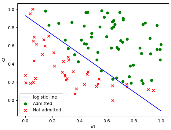
对于样本数据,上面的梯度下降并不是非常有效,无论是否预处理数据(归一化或其他方法),都必须反复调整学习率和迭代次数。如果学习率过大,算法将不会收敛;如果过小,算法收敛的十分缓慢,需要增加迭代次数。代码中的参数最终将使算法收敛于0.203。
Sklearn
 from sklearn.linear_model import LogisticRegression

 import numpy as np

 if __name__ == '__main__':

     train_datas = np.loadtxt("ex2data1.txt", delimiter=',')

     X_train = train_datas[:,[0, 1]]

     Y_train = train_datas[:,[2]]

     logistic = LogisticRegression()

     logistic.fit(X_train, Y_train)

     theta = [logistic.intercept_[0], logistic.coef_[0]]

     print(theta)
参考:
Ng视频《Logistic Regression》
周志华《机器学习》
《机器学习导论》
Peter Flach《机器学习》
作者:我是8位的
出处:http://www.cnblogs.com/bigmonkey
本文以学习、研究和分享为主,如需转载,请联系本人,标明作者和出处,非商业用途!
扫描二维码关注公众号“我是8位的”

ML(4)——逻辑回归的更多相关文章
- [机器学习] Coursera ML笔记 - 逻辑回归(Logistic Regression)
引言 机器学习栏目记录我在学习Machine Learning过程的一些心得笔记,涵盖线性回归.逻辑回归.Softmax回归.神经网络和SVM等等.主要学习资料来自Standford Andrew N ...
- 大叔学ML第五:逻辑回归
目录 基本形式 代价函数 用梯度下降法求\(\vec\theta\) 扩展 基本形式 逻辑回归是最常用的分类模型,在线性回归基础之上扩展而来,是一种广义线性回归.下面举例说明什么是逻辑回归:假设我们有 ...
- Spark ML逻辑回归
import org.apache.log4j.{Level, Logger} import org.apache.spark.ml.classification.LogisticRegression ...
- ML 逻辑回归 Logistic Regression
逻辑回归 Logistic Regression 1 分类 Classification 首先我们来看看使用线性回归来解决分类会出现的问题.下图中,我们加入了一个训练集,产生的新的假设函数使得我们进行 ...
- Matlab实现线性回归和逻辑回归: Linear Regression & Logistic Regression
原文:http://blog.csdn.net/abcjennifer/article/details/7732417 本文为Maching Learning 栏目补充内容,为上几章中所提到单参数线性 ...
- Stanford机器学习---第三讲. 逻辑回归和过拟合问题的解决 logistic Regression & Regularization
原文:http://blog.csdn.net/abcjennifer/article/details/7716281 本栏目(Machine learning)包括单参数的线性回归.多参数的线性回归 ...
- Spark机器学习(2):逻辑回归算法
逻辑回归本质上也是一种线性回归,和普通线性回归不同的是,普通线性回归特征到结果输出的是连续值,而逻辑回归增加了一个函数g(z),能够把连续值映射到0或者1. MLLib的逻辑回归类有两个:Logist ...
- Spark LogisticRegression 逻辑回归之建模
导入包 import org.apache.spark.sql.SparkSession import org.apache.spark.sql.Dataset import org.apache.s ...
- pyspark 逻辑回归程序
http://www.qqcourse.com/forum.php?mod=viewthread&tid=3688 [很重要]:http://spark.apache.org/docs/lat ...
随机推荐
- SUSE_LINUX 11 SP3 安装 IBM MQ 7.5
0.环境介绍 mq7.5 suse linux 11 1. 上传安装包 上传安装包到 softWare/CI79IML.tar.gz 2. 安装证书 sh ./mqlicense.sh 输入 1 同意 ...
- SharePoint Framework 企业向导(一)
博客地址:http://blog.csdn.net/FoxDave 简介 SharePoint Framework(SPFx)是一个新的SharePoint用户接口扩展的开发模型,它用来补充现有的 ...
- Oracle hint手动优化
例子 select/*+FULL(fortest)*/ * from fortest where id = 2000000 //使用0.70s时间 select* from fortest where ...
- day 36 关于io模型的问题 阻塞 和多路复用
# from gevent import spawn,monkey;monkey.patch_all()# from socket import *# def server(ip,port):# se ...
- mysql创建用户并给用户分配权限
1.登录Mysql [root@xufeng Desktop]# mysql -u root -pEnter password: Welcome to the MySQL monitor. Comma ...
- Python 属性
class Person: def __init__(self, name, gender, birth): self.name = name self.gender = gender self.bi ...
- wx小程序 使用字体
1.下载项目下的字体库 2.解压复制iconfont.css中的代码到,小程序 app.wxss 3.使用: //icon-begindate表示开始时间的图标 <text class=&quo ...
- 笔记:Oracle查询重复数据并删除,只保留一条记录
1.查找表中多余的重复记录,重复记录是根据单个字段(Id)来判断 select * from 表 where Id in (select Id from 表 group byId having cou ...
- mysql 数据查询全讲
数据查询 涉及到DQL(Data Query Language)是sql语句的一类 本文全面介绍了mysql下 select 语句的各种查询方式:普通查询,模糊查询,查询排序,分页查询,聚合函数查询 ...
- pip install GitHub package
/********************************************************************************* * pip install Git ...