mnist手写数字识别——深度学习入门项目（tensorflow+keras+Sequential模型）

前言

今天记录一下深度学习的另外一个入门项目——《mnist数据集手写数字识别》，这是一个入门必备的学习案例，主要使用了tensorflow下的keras网络结构的Sequential模型，常用层的Dense全连接层、Activation激活层和Reshape层。还有其他方法训练手写数字识别模型，可以基于pytorch实现的，《Pytorch实现基于卷积神经网络的面部表情识别(详细步骤)》 这篇就是基于pytorch实现，pytorch里也封装了mnist的数据集，实现方法应该类似，正在学习中……
这一篇记录则是基于keras的Sequential模型实现的。

项目步骤

前言

　　 1、mnist手写数字真面目

　　　　1.1、mnist（集成）数据集

　　　　1.2、mnist数据集（训练测试数据与标签分离）

　　 2、Sequential模型训练

　　 写在后面

1、mnist手写数字真面目

我们使用离线下载的数据集进行导入，一定程度上解决了从远程加载数据缓慢的问题，这里有两种数据集提供给大家，分别是：

1. mnist.npz数据集
   它是把手写数字的图像数据和对应标签集成在一起，而且训练集与测试集也在里面，使用的时候无需拆分文件，只需要简单代码划分数据，可直接下载本地 mnist手写数字识别数据集npz文件.zip
2. mnist.zip数据集
   它包含了两个压缩包，分别是训练集和测试集（文件名：mnist_traint_data.zip和mnist_test_data.zip），每个数据集解压后里面分别是数据和对应的标签，所以最后由4个文件，可直接下载本地 mnist训练数据+测试数据(手写数字识别).zip

　　1.1、mnist.npz（集成）数据集

下载好mnist手写数字识别数据集npz文件.zip之后，解压得到mnist.npz之后，我们这里开始写代码看看手写数字图像的真面目。
显示图像代码：

import numpy as np
import matplotlib.pyplot as plt

def load_mnist(): # 自定义加载数据
    path = r'D:\mnist_data\mnist.npz'  # 放置mnist.npz的目录。注意斜杠
    f = np.load(path)
    x_train, y_train = f['x_train'], f['y_train']  # 代码实现分离数据集里面的训练集和测试集以及对应标签
    x_test, y_test = f['x_test'], f['y_test']  # x_train为训练数据，y_train为对应标签

    f.close() # 关闭文件
    return (x_train, y_train), (x_test, y_test)

def main():
    (X_train, y_train_label), (test_image, test_label) = load_mnist() #后续可以显示训练数据的数字或者测试数据的

    fig, ax = plt.subplots(nrows=5, ncols=5, sharex=True, sharey=True)  # 显示图像
    ax = ax.flatten()
    for i in range(25):
        img = X_train[i].reshape(28, 28)
        # img = X_train[y_train_label == 8][i].reshape(28, 28)  # 显示标签为8的数字图像
        ax[i].set_title(y_train_label[i])
        ax[i].imshow(img, cmap='Greys', interpolation='nearest')
    ax[0].set_xticks([])
    ax[0].set_yticks([])
    plt.tight_layout()
    plt.show()

if __name__ == '__main__':
    main()

效果如下：

也可以花样输出：
代码：

import numpy as np
import matplotlib.pyplot as plt

def load_mnist():
    path = r'D:\mnist_data\mnist.npz'  # 放置mnist.npz的目录。注意斜杠
    f = np.load(path)
    x_train, y_train = f['x_train'], f['y_train']  # 代码实现分离数据集里面的训练集和测试集以及对应标签
    x_test, y_test = f['x_test'], f['y_test']  # x_train为训练数据，y_train为对应标签

    f.close() # 关闭文件
    return (x_train, y_train), (x_test, y_test)

def main():
    (X_train, y_train_label), (test_image, test_label) = load_mnist()
    plt.subplot(221)#显示图像
    plt.imshow(X_train[0], cmap=plt.get_cmap('Accent'))
    plt.subplot(222)
    plt.imshow(X_train[1], cmap=plt.get_cmap('gray'))
    plt.subplot(223)
    plt.imshow(X_train[2], cmap=plt.get_cmap('Blues'))
    plt.subplot(224)
    plt.imshow(X_train[3], cmap=plt.get_cmap('Oranges'))
    plt.show()

if __name__ == '__main__':
    main()

图像显示：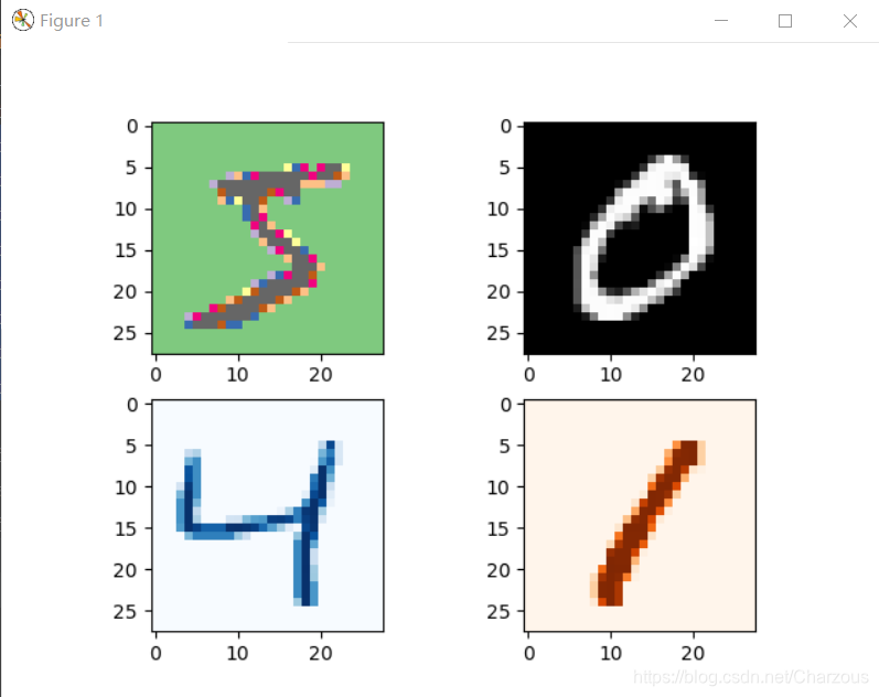

　　1.2、mnist数据集（训练测试数据与标签分离）

这里介绍第二中方法，也就是数据集是分离的，下载好mnist训练数据+测试数据(手写数字识别).zip之后，解压得到文件如图：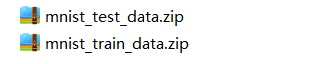

进去解压得到：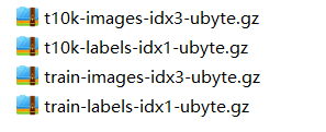

可以看到分别是训练集和测试集，包括数据和标签。
这种方法比较麻烦，没想到吧！^_ ^ ，大家可以选择第一种步骤简单
最后得到：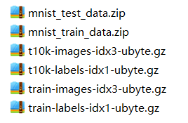

导入时候需要用到的是这些.gz文件。
显示图像代码：

import gzip
import os
import numpy as np
import matplotlib.pyplot as plt

local_file = 'D:\mnist_data'
files = ['train-images-idx3-ubyte.gz', 'train-labels-idx1-ubyte.gz',
         't10k-images-idx3-ubyte.gz', 't10k-labels-idx1-ubyte.gz']

def load_local_mnist(filename):# 加载文件
    paths = []
    file_read = []
    for file in files:
        paths.append(os.path.join(filename, file))
    for path in paths:
        file_read.append(gzip.open(path, 'rb'))
    # print(file_read)

    train_labels = np.frombuffer(file_read[1].read(), np.uint8, offset=8)#文件读取以及格式转换
    train_images = np.frombuffer(file_read[0].read(), np.uint8, offset=16) \
        .reshape(len(train_labels), 28, 28)
    test_labels = np.frombuffer(file_read[3].read(), np.uint8, offset=8)
    test_images = np.frombuffer(file_read[2].read(), np.uint8, offset=16) \
        .reshape(len(test_labels), 28, 28)
    return (train_images, train_labels), (test_images, test_labels)

def main():
    (x_train, y_train), (x_test, y_test) = load_local_mnist(local_file)

    fig, ax = plt.subplots(nrows=6, ncols=6, sharex=True, sharey=True)#显示图像
    ax = ax.flatten()
    for i in range(36):
        img=x_test[i].reshape(28,28)
        # img = x_train[y_train == 8][i].reshape(28, 28)  # 显示标签为8的数字图像
        ax[i].set_title(y_train[i])
        ax[i].imshow(img, cmap='Greys', interpolation='nearest')
    ax[0].set_xticks([])
    ax[0].set_yticks([])
    plt.tight_layout()
    plt.show()

if __name__ == '__main__':
    main()

输出结果：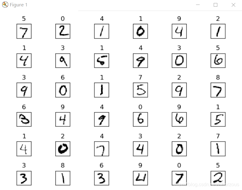

2、Sequential模型训练

这里实现主要使用了tensorflow下的keras网络结构的Sequential模型，常用层的Dense全连接层、Activation激活层和Reshape层。tensorflow安装有问题可参考《初入机器学习，安装tensorflow包等问题总结》
模型比较简单，网络搭建以及模型选择的损失函数、优化器可见代码。

import numpy as np
import os
import gzip
from tensorflow import keras
from tensorflow.keras.optimizers import SGD
from tensorflow_core.python.keras.utils import np_utils
from tensorflow.keras.layers import Dense, Dropout, Activation

local_file = 'D:\mnist_data'
files = ['train-images-idx3-ubyte.gz', 'train-labels-idx1-ubyte.gz',
         't10k-images-idx3-ubyte.gz', 't10k-labels-idx1-ubyte.gz']

def load_local_mnist(filename):  # 加载文件
    paths = []
    file_read = []
    for file in files:
        paths.append(os.path.join(filename, file))
    for path in paths:
        file_read.append(gzip.open(path, 'rb'))
    # print(file_read)

    train_labels = np.frombuffer(file_read[1].read(), np.uint8, offset=8)  # 文件读取以及格式转换
    train_images = np.frombuffer(file_read[0].read(), np.uint8, offset=16) \
        .reshape(len(train_labels), 28, 28)
    test_labels = np.frombuffer(file_read[3].read(), np.uint8, offset=8)
    test_images = np.frombuffer(file_read[2].read(), np.uint8, offset=16) \
        .reshape(len(test_labels), 28, 28)
    return (train_images, train_labels), (test_images, test_labels)

def load_data():# 加载模型需要的数据
    (x_train, y_train), (x_test, y_test) = load_local_mnist(local_file)
    number = 10000
    x_train = x_train[0:number]
    y_train = y_train[0:number]
    x_train = x_train.reshape(number, 28 * 28)
    x_test = x_test.reshape(x_test.shape[0], 28 * 28)
    x_train = x_train.astype('float32')
    x_test = x_test.astype('float32')

    y_train = np_utils.to_categorical(y_train, 10)
    y_test = np_utils.to_categorical(y_test, 10)
    x_train = x_train
    x_test = x_test

    x_train = x_train / 255
    x_test = x_test / 255
    return (x_train, y_train), (x_test, y_test)

(X_train, Y_train), (X_test, Y_test) = load_data()
model = keras.Sequential()# 模型选择
model.add(Dense(input_dim=28 * 28, units=690,
                activation='relu'))  # tanh  activation：Sigmoid、tanh、ReLU、LeakyReLU、pReLU、ELU、maxout
model.add(Dense(units=690, activation='relu'))
model.add(Dense(units=690, activation='relu'))  # tanh
model.add(Dense(units=10, activation='relu'))
model.compile(loss='mse', optimizer=SGD(lr=0.1),
              metrics=['accuracy'])  # loss:mse,categorical_crossentropy,optimizer: rmsprop 或 adagrad、SGD（此处推荐）
model.fit(X_train, Y_train, batch_size=100, epochs=20)
result = model.evaluate(X_test, Y_test)
print('TEST ACC:', result[1])

经过稍微调优，发现输入层激活函数使用relu和tanh效果好，其他网络层使用relu。另外，损失函数使用了MSE（均方误差），优化器使用 SGD（随即梯度下降），学习率learning rate调到0.1，度量常用正确率。
参数batch_size=100, epochs=20，增加参数更新以及训练速度。
以上参数以及选择训练效果如下：

使用优化器为adagrad效果：

大家也可以自行各种尝试，优化器和损失函数选择，参数调优等，进一步提高正确率。

这里提供另一种写法，模型构建类似。

import tensorflow as tf
from tensorflow.keras import datasets, layers, optimizers, models, metrics
from tensorflow.keras.optimizers import SGD

import os

os.environ['TF_CPP_MIN_LOG_LEVEL'] = ''  # 忽略tensorflow版本警告
(xs, ys), _ = datasets.mnist.load_data()
print('datasets:', xs.shape, ys.shape, xs.min(), xs.max())

# tf.compat.v1.enable_eager_execution()
tf.enable_eager_execution()
xs = tf.convert_to_tensor(xs, dtype=tf.float32) / 255.
db = tf.data.Dataset.from_tensor_slices((xs, ys))
db = db.batch(100).repeat(20)

network = models.Sequential([layers.Dense(256, activation='relu'),
                             layers.Dense(256, activation='relu'),
                             layers.Dense(256, activation='relu'),
                             layers.Dense(10)])
network.build(input_shape=(None, 28 * 28))
network.summary()

optimizer = optimizers.SGD(lr=0.01)
acc_meter = metrics.Accuracy()# 度量正确率

for step, (x, y) in enumerate(db):

    with tf.GradientTape() as tape:
        # [b, 28, 28] => [b, 784] 784维=24*24
        x = tf.reshape(x, (-1, 28 * 28))#-1的含义，数组新的shape属性应该要与原来的配套，根据剩下的维度计算出数组的另外一个shape属性值。
        # [b, 784] => [b, 10]
        out = network(x)
        # [b] => [b, 10]
        y_onehot = tf.one_hot(y, depth=10)  # 独热编码，y = 0 对应的输出是[1,0,0,0,0,0,0,0,0,0]，范围0-9，depth深度10层表示10个数字
        # [b, 10]
        loss = tf.square(out - y_onehot)# 计算模型预测与实际的损失
        # [b]
        loss = tf.reduce_sum(loss) / 32

    acc_meter.update_state(tf.argmax(out, axis=1), y)
    grads = tape.gradient(loss, network.trainable_variables)# 计算梯度
    optimizer.apply_gradients(zip(grads, network.trainable_variables))

    if step % 200 == 0:
        print(step, 'loss:', float(loss), 'acc:', acc_meter.result().numpy())
        acc_meter.reset_states()

最后正确率比上面好一点，如图：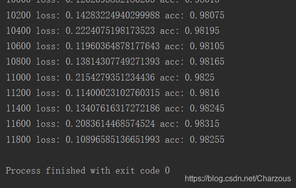

写在后面

经过这次学习，感觉收获了许多，之前只是在理论知识上的理解，现在配合代码实践，模型训练，理解更加深刻，还存在不足，欢迎大家指正交流，这个过程的详细步骤，希望能帮助跟我一样入门需要的伙伴，记录学习过程，感觉总结一下很好，继续加油！

我的CSDN博客：mnist手写数字识别深度学习入门项目（tensorflow+keras+Sequential模型）
我的博客园：mnist手写数字识别——深度学习入门项目（tensorflow+keras+Sequential模型）

版权声明：本文为博主原创文章，遵循CC 4.0 BY-SA版权协议，转载请附上原文出处链接和本声明。

本文链接：https://blog.csdn.net/Charzous/article/details/107748508