卷积神经网络入门：LeNet5（手写体数字识别）详解

第一张图包括8层LeNet5卷积神经网络的结构图，以及其中最复杂的一层S2到C3的结构处理示意图。



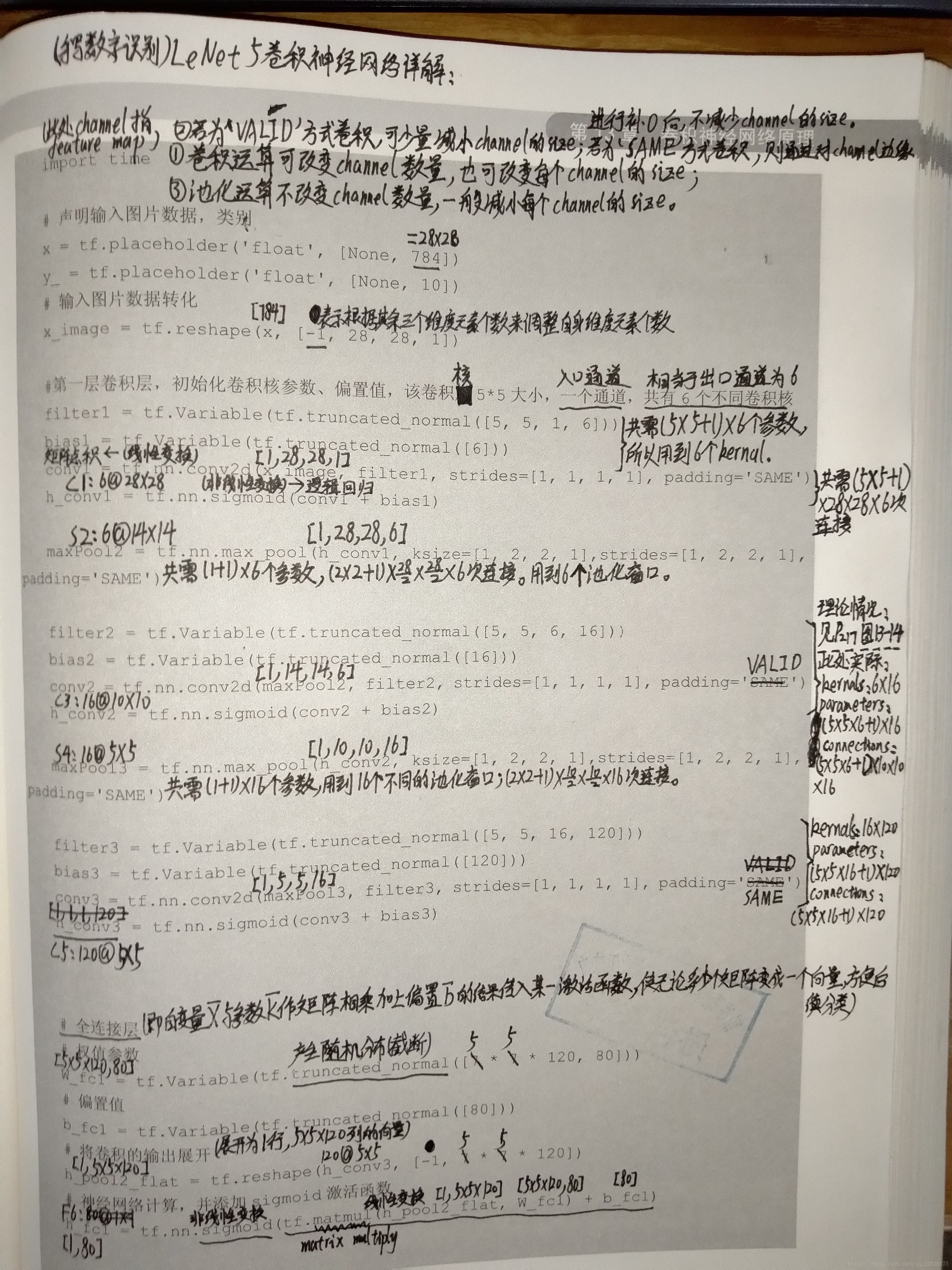
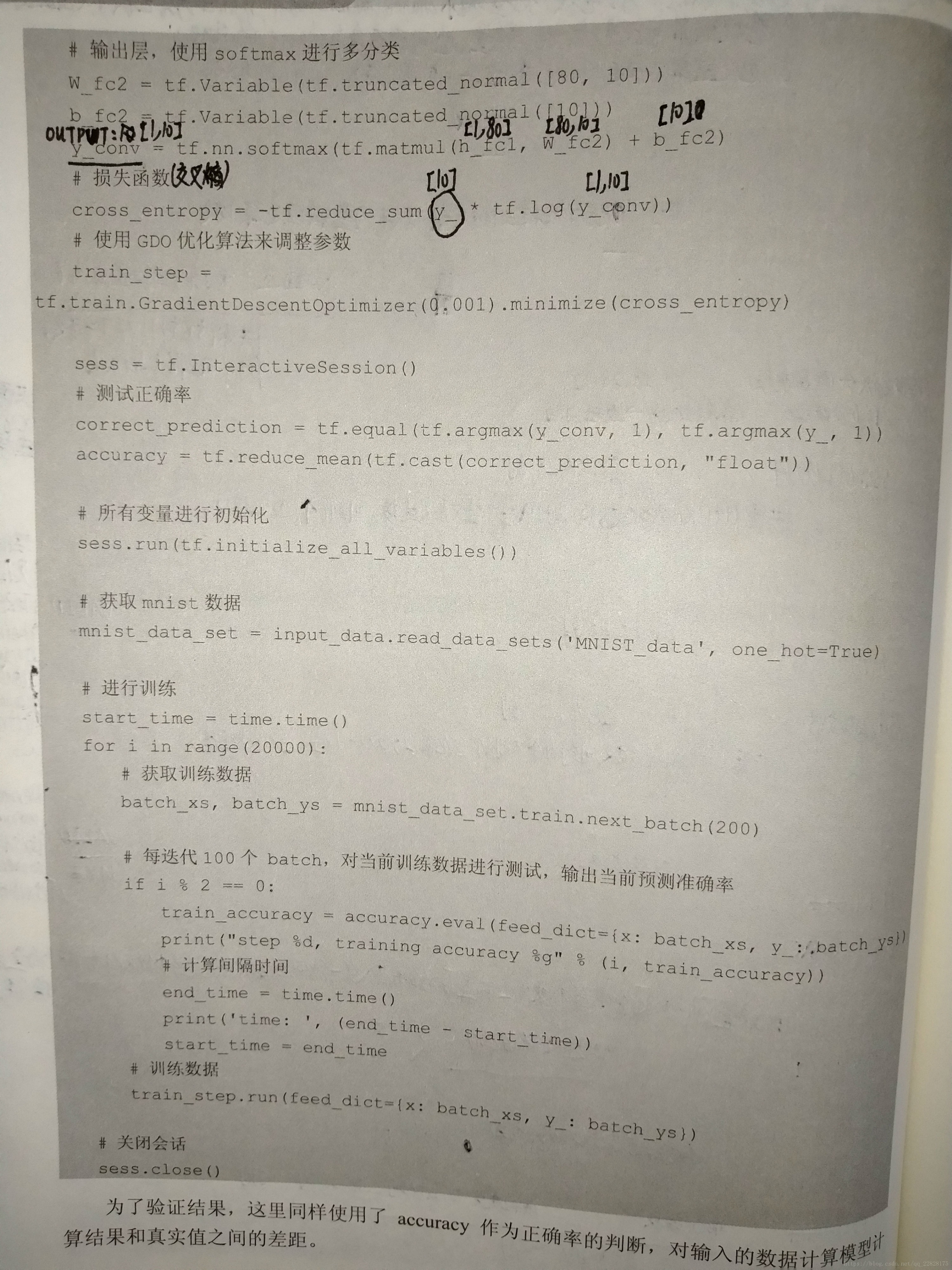
第二张图及第三张图是用tensorflow重写LeNet5网络及其注释。

这是原始的LeNet5网络：

import tensorflow as tf
from tensorflow.examples.tutorials.mnist import input_data
import time

# 声明输入图片数据，类别
x = tf.placeholder('float', [None, 784])
y_ = tf.placeholder('float', [None, 10])
# 输入图片数据转化
x_image = tf.reshape(x, [-1, 28, 28, 1])

#第一层卷积层，初始化卷积核参数、偏置值，该卷积层5*5大小，一个通道，共有6个不同卷积核
filter1 = tf.Variable(tf.truncated_normal([5, 5, 1, 6]))
bias1 = tf.Variable(tf.truncated_normal([6]))
conv1 = tf.nn.conv2d(x_image, filter1, strides=[1, 1, 1, 1], padding='SAME')
h_conv1 = tf.nn.sigmoid(conv1 + bias1)

maxPool2 = tf.nn.max_pool(h_conv1, ksize=[1, 2, 2, 1],strides=[1, 2, 2, 1], padding='SAME')

filter2 = tf.Variable(tf.truncated_normal([5, 5, 6, 16]))
bias2 = tf.Variable(tf.truncated_normal([16]))
conv2 = tf.nn.conv2d(maxPool2, filter2, strides=[1, 1, 1, 1], padding='SAME')
h_conv2 = tf.nn.sigmoid(conv2 + bias2)

maxPool3 = tf.nn.max_pool(h_conv2, ksize=[1, 2, 2, 1],strides=[1, 2, 2, 1], padding='SAME')

filter3 = tf.Variable(tf.truncated_normal([5, 5, 16, 120]))
bias3 = tf.Variable(tf.truncated_normal([120]))
conv3 = tf.nn.conv2d(maxPool3, filter3, strides=[1, 1, 1, 1], padding='SAME')
h_conv3 = tf.nn.sigmoid(conv3 + bias3)

# 全连接层
# 权值参数
W_fc1 = tf.Variable(tf.truncated_normal([7 * 7 * 120, 80]))
# 偏置值
b_fc1 = tf.Variable(tf.truncated_normal([80]))
# 将卷积的产出展开
h_pool2_flat = tf.reshape(h_conv3, [-1, 7 * 7 * 120])
# 神经网络计算，并添加sigmoid激活函数
h_fc1 = tf.nn.sigmoid(tf.matmul(h_pool2_flat, W_fc1) + b_fc1)

# 输出层，使用softmax进行多分类
W_fc2 = tf.Variable(tf.truncated_normal([80, 10]))
b_fc2 = tf.Variable(tf.truncated_normal([10]))
y_conv = tf.nn.softmax(tf.matmul(h_fc1, W_fc2) + b_fc2)
# 损失函数
cross_entropy = -tf.reduce_sum(y_ * tf.log(y_conv))
# 使用GDO优化算法来调整参数
train_step = tf.train.GradientDescentOptimizer(0.001).minimize(cross_entropy)

sess = tf.InteractiveSession()
# 测试正确率
correct_prediction = tf.equal(tf.argmax(y_conv, 1), tf.argmax(y_, 1))
accuracy = tf.reduce_mean(tf.cast(correct_prediction, "float"))

# 所有变量进行初始化
sess.run(tf.initialize_all_variables())

# 获取mnist数据
mnist_data_set = input_data.read_data_sets('MNIST_data', one_hot=True)

# 进行训练
start_time = time.time()
for i in range(20000):
    # 获取训练数据
    batch_xs, batch_ys = mnist_data_set.train.next_batch(200)

    # 每迭代100个 batch，对当前训练数据进行测试，输出当前预测准确率
    if i % 2 == 0:
        train_accuracy = accuracy.eval(feed_dict={x: batch_xs, y_: batch_ys})
        print("step %d, training accuracy %g" % (i, train_accuracy))
        # 计算间隔时间
        end_time = time.time()
        print('time: ', (end_time - start_time))
        start_time = end_time
    # 训练数据
    train_step.run(feed_dict={x: batch_xs, y_: batch_ys})

# 关闭会话
sess.close()

下面是改进后的LeNet5网络：

import tensorflow as tf
from tensorflow.examples.tutorials.mnist import input_data
import time
import matplotlib.pyplot as plt

# 初始化单个卷积核上的权重
def weight_variable(shape):
    initial = tf.truncated_normal(shape, stddev=0.1)
    return tf.Variable(initial)

# 初始化单个卷积核上的偏置值
def bias_variable(shape):
    initial = tf.constant(0.1, shape=shape)
    return tf.Variable(initial)

# 输入特征x，用卷积核W进行卷积运算，strides为卷积核移动步长，
# padding表示是否需要补齐边缘像素使输出图像大小不变
def conv2d(x, W):
    return tf.nn.conv2d(x, W, strides=[1, 1, 1, 1], padding='SAME')

# 对x进行最大池化操作，ksize进行池化的范围，
def max_pool_2x2(x):
    return tf.nn.max_pool(x, ksize=[1, 2, 2, 1], strides=[1, 2, 2, 1], padding='SAME')

sess = tf.InteractiveSession()
# 声明输入图片数据，类别
x = tf.placeholder('float32', [None, 784])
y_ = tf.placeholder('float32', [None, 10])
# 输入图片数据转化
x_image = tf.reshape(x, [-1, 28, 28, 1])

W_conv1 = weight_variable([5, 5, 1, 32])
b_conv1 = bias_variable([32])
h_conv1 = tf.nn.relu(conv2d(x_image, W_conv1) + b_conv1)
h_pool1 = max_pool_2x2(h_conv1)

W_conv2 = weight_variable([5, 5, 32, 64])
b_conv2 = bias_variable([64])
h_conv2 = tf.nn.relu(conv2d(h_pool1, W_conv2) + b_conv2)
h_pool2 = max_pool_2x2(h_conv2)

W_fc1 = weight_variable([7 * 7 * 64, 1024])
# 偏置值
b_fc1 = bias_variable([1024])
# 将卷积的产出展开
h_pool2_flat = tf.reshape(h_pool2, [-1, 7 * 7 * 64])
# 神经网络计算，并添加relu激活函数
h_fc1 = tf.nn.relu(tf.matmul(h_pool2_flat, W_fc1) + b_fc1)

W_fc2 = weight_variable([1024, 128])
b_fc2 = bias_variable([128])
h_fc2 = tf.nn.relu(tf.matmul(h_fc1, W_fc2) + b_fc2)

W_fc3 = weight_variable([128, 10])
b_fc3 = bias_variable([10])
y_conv = tf.nn.softmax(tf.matmul(h_fc2, W_fc3) + b_fc3)
# 代价函数
cross_entropy = -tf.reduce_sum(y_ * tf.log(y_conv))
# 使用Adam优化算法来调整参数
train_step = tf.train.GradientDescentOptimizer(1e-5).minimize(cross_entropy)

# 测试正确率
correct_prediction = tf.equal(tf.argmax(y_conv, 1), tf.argmax(y_, 1))
accuracy = tf.reduce_mean(tf.cast(correct_prediction, "float32"))

# 所有变量进行初始化
sess.run(tf.initialize_all_variables())

# 获取mnist数据
mnist_data_set = input_data.read_data_sets('MNIST_data', one_hot=True)
c = []

# 进行训练
start_time = time.time()
for i in range(1000):
    # 获取训练数据
    batch_xs, batch_ys = mnist_data_set.train.next_batch(200)

    # 每迭代10个 batch，对当前训练数据进行测试，输出当前预测准确率
    if i % 2 == 0:
        train_accuracy = accuracy.eval(feed_dict={x: batch_xs, y_: batch_ys})
        c.append(train_accuracy)
        print("step %d, training accuracy %g" % (i, train_accuracy))
        # 计算间隔时间
        end_time = time.time()
        print('time: ', (end_time - start_time))
        start_time = end_time
    # 训练数据
    train_step.run(feed_dict={x: batch_xs, y_: batch_ys})

sess.close()
plt.plot(c)
plt.tight_layout()