matlab(8) Regularized logistic regression : 不同的λ(0,1,10,100)值对regularization的影响，对应不同的decision boundary\ 预测新的值和计算模型的精度predict.m

不同的λ(0,1,10,100)值对regularization的影响\ 预测新的值和计算模型的精度

%% ============= Part 2: Regularization and Accuracies =============
% Optional Exercise:
% In this part, you will get to try different values of lambda and
% see how regularization affects the decision coundart
%
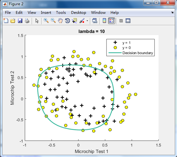
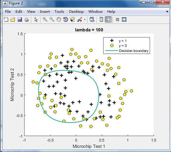
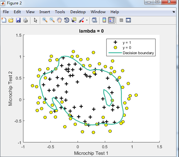
% Try the following values of lambda (0, 1, 10, 100).
%
% How does the decision boundary change when you vary lambda? How does
% the training set accuracy vary?
%

% Initialize fitting parameters
initial_theta = zeros(size(X, 2), 1);

% Set regularization parameter lambda to 1 (you should vary this)
lambda = 1;    %在这里设置λ=(0,1,10,100)

由下图可见，lambda=1时的效果最好，

λ=0时No regularization(overfitting);

λ=100时会too much regularization(underfitting),

% Set Options
options = optimset('GradObj', 'on', 'MaxIter', 400);   %计算gradient,迭代的次数为400次

% Optimize
[theta, J, exit_flag] = ...
fminunc(@(t)(costFunctionReg(t, X, y, lambda)), initial_theta, options);

% Plot Boundary
plotDecisionBoundary(theta, X, y);  %X已经mapFeature过了
hold on;
title(sprintf('lambda = %g', lambda))    % 会在%e和%f中自动选择一种格式，且无后缀0。

% Labels and Legend
xlabel('Microchip Test 1')
ylabel('Microchip Test 2')

legend('y = 1', 'y = 0', 'Decision boundary')
hold off;

% Compute accuracy on our training set
p = predict(theta, X);

fprintf('Train Accuracy: %f\n', mean(double(p == y)) * 100);

plotDecisionBoundary.m文件

function plotDecisionBoundary(theta, X, y)
%PLOTDECISIONBOUNDARY Plots the data points X and y into a new figure with
%the decision boundary defined by theta
% PLOTDECISIONBOUNDARY(theta, X,y) plots the data points with + for the
% positive examples and o for the negative examples. X is assumed to be
% a either
% 1) Mx3 matrix, where the first column is an all-ones column for the
% intercept.
% 2) MxN, N>3 matrix, where the first column is all-ones

% Plot Data
plotData(X(:,2:3), y);
hold on

if size(X, 2) <= 3
% Only need 2 points to define a line, so choose two endpoints
   plot_x = [min(X(:,2))-2, max(X(:,2))+2];

% Calculate the decision boundary line
   plot_y = (-1./theta(3)).*(theta(2).*plot_x + theta(1));

% Plot, and adjust axes for better viewing
   plot(plot_x, plot_y)

% Legend, specific for the exercise
   legend('Admitted', 'Not admitted', 'Decision Boundary')
   axis([30, 100, 30, 100])
else      %X已经mapFeature过了(有28个features)，调用这部分的程序
% Here is the grid range
   u = linspace(-1, 1.5, 50);
   v = linspace(-1, 1.5, 50);

z = zeros(length(u), length(v));
% Evaluate z = theta*x over the grid
for i = 1:length(u)
    for j = 1:length(v)
       z(i,j) = mapFeature(u(i), v(j))*theta;
    end
end
z = z'; % important to transpose z before calling contour

% Plot z = 0
% Notice you need to specify the range [0, 0]
contour(u, v, z, [0, 0], 'LineWidth', 2)    %画等值线.contour(X,Y,Z,[v v]) to draw contours for the single level v.
end  %if size(X, 2) <= 3  else的end
hold off

end

predict.m文件

function p = predict(theta, X)
%PREDICT Predict whether the label is 0 or 1 using learned logistic
%regression parameters theta
% p = PREDICT(theta, X) computes the predictions for X using a
% threshold at 0.5 (i.e., if sigmoid(theta'*x) >= 0.5, predict 1)

m = size(X, 1); % Number of training examples

% You need to return the following variables correctly
p = zeros(m, 1);

% ====================== YOUR CODE HERE ======================
% Instructions: Complete the following code to make predictions using
% your learned logistic regression parameters.
% You should set p to a vector of 0's and 1's
%
for i=1:m
    if sigmoid(X(i,:) * theta) >=0.5
        p(i) = 1;
    else
        p(i) = 0;
    end
end

% =========================================================================

end