GMM实战

一道作业题：

https://www.kaggle.com/c/speechlab-aug03

就是给你训练集，验证集，要求用GMM（混合高斯模型）预测 测试集的分类，这是个2分类的问题。

$ head train.txt dev.txt test.txt
==> train.txt <==
1.124586 1.491173
2.982154 0.275734
-0.367243 0.068235
1.216709 -0.804729
3.077832 0.307613
1.165453 1.627965
0.737648 1.055470
0.838988 1.355942
1.452510 -0.056967
-0.570093 -0.355338 

==> dev.txt <==
0.900742 1.933559
3.112402 -0.817857
0.989450 1.605954
0.759107 -1.214189
1.433045 -0.986053
1.072825 1.654026
2.174214 0.638420
1.135233 -1.055797
-0.328072 -0.091407
1.220020 1.116177 

==> test.txt <==
0.916983 0.353964
1.921382 1.958336
1.822650 2.328900
-0.786640 -0.059369
1.018302 1.406017
0.660574 0.847398
2.747331 0.910621
0.662462 1.935314
2.955916 -0.317031
-0.213735 0.126742

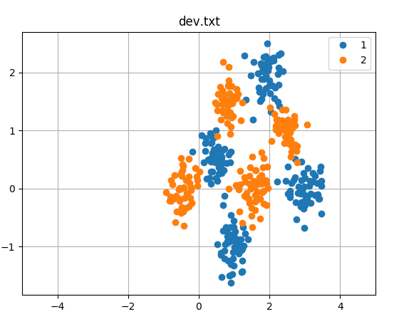
这里我已经把图画出来了，因为特征是2维的，所以可以用平面上的点来表示，不同的颜色代表不同的分类。

这个题的思路就是：用两个GMM来做，每个GMM有4个组分，最后要看属于哪一类，就看两个GMM模型的概率，谁高就属于哪一类。

要对两个GMM模型做初始化，在这里用Kmeans来做初始化，比随机初始化要好。

1.Kmeans初始化：

# from numpy import *
import numpy as np
import matplotlib.pyplot as plt
import os

use_new_data=0
#-------------------new-----------------
if use_new_data:
    colour=['lightblue','sandybrown']
    _path='/home/dahu/myfile/tianchi/kaggle/gmm_em/my_test/new'
    train_file=os.path.join(_path,'train.txt1')
    dev_file=os.path.join(_path,'dev.txt1')
    test_file=os.path.join(_path,'test.txt1')

#-------------------old-----------------
else :
    _path='/home/dahu/myfile/tianchi/kaggle/gmm_em/my_test/old'
    train_file=os.path.join(_path,'train.txt')
    dev_file=os.path.join(_path,'dev.txt')
    test_file=os.path.join(_path,'test.txt')

feature_num=2
n_classes = 4

plt.rc('figure', figsize=(10, 6))
def loadDataSet(fileName):  # 解析文件，按tab分割字段，得到一个浮点数字类型的矩阵
    dataMat = []              # 文件的最后一个字段是类别标签
    fr = open(fileName)
    for line in fr.readlines():
        curLine = line.strip().split(' ')
#         fltLine = map(float, curLine)    # 将每个元素转成float类型
        fltLine=[float(i) for i in curLine]
        dataMat.append(fltLine)
    return dataMat

# 计算欧几里得距离
def distEclud(vecA, vecB):
    return np.sqrt(np.sum(np.power(vecA - vecB, 2))) # 求两个向量之间的距离

# 构建聚簇中心，取k个(此例中k=4)随机质心
def randCent(dataSet, k):
    np.random.seed(1)
    n = np.shape(dataSet)[1]
    centroids = np.mat(np.zeros((k,n)))   # 每个质心有n个坐标值，总共要k个质心
    for j in range(n):
        minJ = min(dataSet[:,j])
        maxJ = max(dataSet[:,j])
        rangeJ = float(maxJ - minJ)
        centroids[:,j] = minJ + rangeJ * np.random.rand(k, 1)
    return centroids

# k-means 聚类算法
def kMeans(dataSet, k, distMeans =distEclud, createCent = randCent):
    '''
    :param dataSet:  没有lable的数据集  (本例中是二维数据)
    :param k:  分为几个簇
    :param distMeans:    计算距离的函数
    :param createCent:   获取k个随机质心的函数
    :return: centroids： 最终确定的 k个 质心
            clusterAssment:  该样本属于哪类  及  到该类质心距离
    '''
    m = np.shape(dataSet)[0]   #m=80,样本数量
    clusterAssment = np.mat(np.zeros((m,2)))
    # clusterAssment第一列存放该数据所属的中心点，第二列是该数据到中心点的距离，
    centroids = createCent(dataSet, k)
    clusterChanged = True   # 用来判断聚类是否已经收敛
    while clusterChanged:
        clusterChanged = False;
        for i in range(m):  # 把每一个数据点划分到离它最近的中心点
            minDist = np.inf; minIndex = -1;
            for j in range(k):
                distJI = distMeans(centroids[j,:], dataSet[i,:])
                if distJI < minDist:
                    minDist = distJI; minIndex = j  # 如果第i个数据点到第j个中心点更近，则将i归属为j
            if clusterAssment[i,0] != minIndex:
                clusterChanged = True  # 如果分配发生变化，则需要继续迭代
            clusterAssment[i,:] = minIndex,minDist**2   # 并将第i个数据点的分配情况存入字典
        # print centroids
        for cent in range(k):   # 重新计算中心点
#             ptsInClust = dataSet[clusterAssment.A[:,0]==cent]
            ptsInClust = dataSet[np.nonzero(clusterAssment[:,0].A == cent)[0]]
            centroids[cent,:] = np.mean(ptsInClust, axis = 0)  # 算出这些数据的中心点
    return centroids, clusterAssment
# --------------------测试----------------------------------------------------
# 用测试数据及测试kmeans算法

data=np.mat(loadDataSet(train_file))
# data=np.mat(loadDataSet('/home/dahu/myfile/my_git/pytorch_learning/pytorch_lianxi/gmm_em.lastyear/train.txt'))
# print(data)
kmeans=[]
colors = ['lightblue','sandybrown']

for i in [1,2]:
    datMat = data[np.nonzero(data[:,feature_num].A == i)[0]]  #选取某一标注的所有样例
#     datMat = data[data.A[:,2]==i]
#     print(datMat)
    myCentroids,clustAssing = kMeans(datMat,n_classes)
    print('Kmeans 中心点坐标展示')
    print(myCentroids)
    x=np.array(datMat[:,0]).ravel()
    y=np.array(datMat[:,1]).ravel()
    plt.scatter(x,y, marker='o',color=colors[i-1],label=i)
    xcent=np.array(myCentroids[:,0]).ravel()
    ycent=np.array(myCentroids[:,1]).ravel()
    plt.scatter(xcent, ycent, marker='x', color='r', s=50)
#     print(myCentroids[:,:2])
    kmeans.append(myCentroids[:,:feature_num])
plt.legend(scatterpoints=1, loc='lower right', prop=dict(size=12))
plt.title('kmeans get center')
plt.show()

kmeans的方法之前的博客已经说了，方法是一样的，在这里，已经把分类和各组分的中心点已经标出了。

kmeans找到的中心点，我们准备用来作为GMM的初始化。

2.GMM训练

f_train=open(train_file,'r')
f_dev=open(dev_file,'r')

x_train=[]
Y_train=[]
x_test=[]
Y_test=[]
for line in f_train:
    a=line.split(' ')
    x_train.append([float(i) for i in a[:feature_num]])
    Y_train.append(int(a[-1]))
X_train=np.array(x_train)
y_train=np.array(Y_train)

for line in f_dev:
    a=line.split(' ')
    x_test.append([float(i) for i in a[:feature_num]])
    Y_test.append(int(a[-1]))
X_test=np.array(x_test)
y_test=np.array(Y_test)

c=[X_train,y_train,X_test,y_test]
# print(X_train[:5],y_train[:5],'\n\n',X_test[:5],y_test[:5],'\n',type(X_train))
# print(X_train[y_train==1])
x1=X_train[y_train==1]
x2=X_train[y_train==2]
xt1=X_test[y_test==1]
xt2=X_test[y_test==2]

print(x1[:5],x1.shape)
# for i in c:
#     print(i.shape)

# --------------------------GMM----------------------------------------------------
# 在这里准备开始搞GMM了，这里用了2个GMM模型
estimator1 = GaussianMixture(n_components=n_classes,
                   covariance_type='full', max_iter=200, random_state=0,tol=1e-5)
estimator2 = GaussianMixture(n_components=n_classes,
                   covariance_type='full', max_iter=200, random_state=0,tol=1e-5)
# estimator.means_init = np.array([X_train[y_train == i+1].mean(axis=0)
#                                     for i in range(n_classes)])

estimator1.means_init = np.array(kmeans[0])    #在这里初始化的，这个值就是我们之前kmeans得到的
estimator2.means_init = np.array(kmeans[1])

# estimator.fit(X_train)
estimator1.fit(x1)
estimator2.fit(x2)

x1_p= np.exp(estimator1.score_samples(X_train))
x2_p= np.exp(estimator2.score_samples(X_train))

# 写了两个函数，一个是预测分类的，其实就是根据 哪个GMM模型的得分高，就是哪一类  这样来分类的， 另一个是根据分类结果，和标注对比，算一个准确率
def predict(x1test_p,x2test_p):
    res=[]
    for i in range(x1test_p.shape[0]):
        if x1test_p[i]>x2test_p[i]:
            res.append(1)
        else:
            res.append(2)
    res=np.array(res)
    return res

def calculate_accuracy(x1test_p,x2test_p,y_test):
    res=predict(x1test_p,x2test_p)
    test_accuracy = np.mean(res.ravel() == y_test.ravel()) * 100
    return test_accuracy

print('开发集train准确率',calculate_accuracy(x1_p,x2_p,y_train))

print('-'*60)

x1test_p=np.exp(estimator1.score_samples(X_test))
x2test_p=np.exp(estimator2.score_samples(X_test))
# print(x1test_p[:5],x1test_p.shape)
# print(x2test_p[:5],x2test_p.shape)
# print(y_test[:5],y_test.shape)

print('验证集dev准确率',calculate_accuracy(x1test_p,x2test_p,y_test))

[[ 2.982154  0.275734]
 [ 1.216709 -0.804729]
 [ 3.077832  0.307613]
 [ 0.710813  0.241071]
 [ 0.599696  0.490842]] (, )
开发集train准确率 98.375
------------------------------------------------------------
验证集dev准确率 97.875

当然这里算 测试集 的 分类，我没有贴上去啊，最后提交的时候，准确率是98% ，当然前面还有得分更高的。。。

最后

经数学帝的提醒，对于 确定 是哪一个分类  这一块的描述不够准确，重新描述一下：

a.我们求的2个GMM的概率其实是 p(x|y=1)  ,p(x|y=2) ，在给定分类情况下，x的概率

b.而我们需要的是p(y=1|x) ,p(y=2|x) ，已经知道是x了，求是哪个分类的概率。

两个不是同一个东西，需要转化一下： p(y=1|x) = p(x|y=1)*p(y=1)/p(x)     ,  p(y=2|x) = p(x|y=2)*p(y=2)/p(x)

分母p(x)是一样的，可以约掉，分子上还有一个p(y=1)  和 p(y=2)  这是先验概率,在题目中，分类1和分类2的数量是一样多的，所以我们求 a ，能反应出我们求b ，如果题目中不一样，还要把它考虑进去。