课程二(Improving Deep Neural Networks: Hyperparameter tuning, Regularization and Optimization)，第二周（Optimization algorithms） —— 2.Programming assignments:Optimization

Optimization

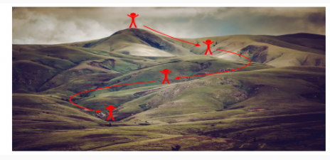
Welcome to the optimization's programming assignment of the hyper-parameters tuning specialization. There are many different optimization algorithms you could be using to get you to the minimal cost. Similarly, there are many different paths down this hill to the lowest point.

By completing this assignment you will:

- Understand the intuition (直觉)between Adam and RMS prop

- Recognize the importance of mini-batch gradient descent

- Learn the effects of momentum on the overall performance of your model

This assignment prepares you well for the upcoming assignment. Take your time to complete it and make sure you get the expected outputs when working through the different exercises. In some code blocks, you will find a "#GRADED FUNCTION: functionName" comment. Please do not modify it. After you are done, submit your work and check your results. You need to score 80% to pass. Good luck :) !

-----------------------------------------------------------------------------------------------------------------

Optimization Methods

Until now, you've always used Gradient Descent to update the parameters and minimize the cost. In this notebook, you will learn more advanced optimization methods that can speed up learning and perhaps even get you to a better final value for the cost function. Having a good optimization algorithm can be the difference between waiting days vs. just a few hours to get a good result.

Gradient descent goes "downhill" on a cost function J. Think of it as trying to do this:

Figure 1 : Minimizing the cost is like finding the lowest point in a hilly landscape

（最小化成本函数就像在丘陵景观中寻找最低点）
At each step of the training, you update your parameters following a certain direction to try to get to the lowest possible point.

Notations: As usual, for any variable a.

To get started, run the following code to import the libraries you will need.

【code】

import numpy as np
import matplotlib.pyplot as plt
import scipy.io
import math
import sklearn
import sklearn.datasets

from opt_utils import load_params_and_grads, initialize_parameters, forward_propagation, backward_propagation
from opt_utils import compute_cost, predict, predict_dec, plot_decision_boundary, load_dataset
from testCases import *

%matplotlib inline
plt.rcParams['figure.figsize'] = (7.0, 4.0) # set default size of plots
plt.rcParams['image.interpolation'] = 'nearest'
plt.rcParams['image.cmap'] = 'gray'

1 - Gradient Descent

A simple optimization method in machine learning is gradient descent (GD). When you take gradient steps with respect to all mm examples on each step, it is also called Batch Gradient Descent.

Warm-up exercise: Implement the gradient descent update rule. The gradient descent rule is, for l=1,...,L:

where L is the number of layers and αα is the learning rate. All parameters should be stored in the parameters dictionary. Note that the iterator l starts at 0 in the for loop while the first parameters are W^[1] and b^[1]. You need to shift l to l+1 when coding.

【code】

# GRADED FUNCTION: update_parameters_with_gd

def update_parameters_with_gd(parameters, grads, learning_rate):
    """
    Update parameters using one step of gradient descent

    Arguments:
    parameters -- python dictionary containing your parameters to be updated:
                    parameters['W' + str(l)] = Wl
                    parameters['b' + str(l)] = bl
    grads -- python dictionary containing your gradients to update each parameters:
                    grads['dW' + str(l)] = dWl
                    grads['db' + str(l)] = dbl
    learning_rate -- the learning rate, scalar.

    Returns:
    parameters -- python dictionary containing your updated parameters
    """

    L = len(parameters) // 2 # number of layers in the neural networks

    # Update rule for each parameter
    for l in range(L):
        ### START CODE HERE ### (approx. 2 lines)
        parameters["W" + str(l+1)] = parameters['W' + str(l+1)]-  learning_rate * grads['dW' + str(l+1)]
        parameters["b" + str(l+1)] =  parameters['b' + str(l+1)] -  learning_rate * grads['db' + str(l+1)]
        ### END CODE HERE ###

    return parameters

parameters, grads, learning_rate = update_parameters_with_gd_test_case()

parameters = update_parameters_with_gd(parameters, grads, learning_rate)
print("W1 = " + str(parameters["W1"]))
print("b1 = " + str(parameters["b1"]))
print("W2 = " + str(parameters["W2"]))
print("b2 = " + str(parameters["b2"]))

【result】

W1 = [[ 1.63535156 -0.62320365 -0.53718766]
 [-1.07799357  0.85639907 -2.29470142]]
b1 = [[ 1.74604067]
 [-0.75184921]]
W2 = [[ 0.32171798 -0.25467393  1.46902454]
 [-2.05617317 -0.31554548 -0.3756023 ]
 [ 1.1404819  -1.09976462 -0.1612551 ]]
b2 = [[-0.88020257]
 [ 0.02561572]
 [ 0.57539477]]

Expected Output:

W1	[[ 1.63535156 -0.62320365 -0.53718766] [-1.07799357 0.85639907 -2.29470142]]
b1	[[ 1.74604067] [-0.75184921]]
W2	[[ 0.32171798 -0.25467393 1.46902454] [-2.05617317 -0.31554548 -0.3756023 ] [ 1.1404819 -1.09976462 -0.1612551 ]]
b2	[[-0.88020257] [ 0.02561572] [ 0.57539477]]

A variant of this is Stochastic Gradient Descent (SGD), which is equivalent to mini-batch gradient descent where each mini-batch has just 1 example. The update rule that you have just implemented does not change. What changes is that you would be computing gradients on just one training example at a time, rather than on the whole training set. The code examples below illustrate the difference between stochastic gradient descent and (batch) gradient descent.

• (Batch) Gradient Descent:

X = data_input
Y = labels
parameters = initialize_parameters(layers_dims)
for i in range(0, num_iterations):
    # Forward propagation
    a, caches = forward_propagation(X, parameters)
    # Compute cost.
    cost = compute_cost(a, Y)
    # Backward propagation.
    grads = backward_propagation(a, caches, parameters)
    # Update parameters.
    parameters = update_parameters(parameters, grads)

• Stochastic Gradient Descent:

X = data_input
Y = labels
parameters = initialize_parameters(layers_dims)
for i in range(0, num_iterations):
    for j in range(0, m):
        # Forward propagation
        a, caches = forward_propagation(X[:,j], parameters)
        # Compute cost
        cost = compute_cost(a, Y[:,j])
        # Backward propagation
        grads = backward_propagation(a, caches, parameters)
        # Update parameters.
        parameters = update_parameters(parameters, grads)

In Stochastic Gradient Descent, you use only 1 training example before updating the gradients. When the training set is large, SGD can be faster. But the parameters will "oscillate" toward the minimum rather than converge smoothly. Here is an illustration of this:

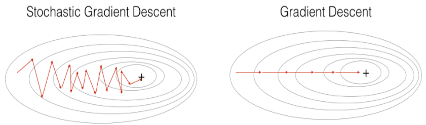
Figure 1 : SGD vs GD
"+" denotes a minimum of the cost. SGD leads to many oscillations to reach convergence. But each step is a lot faster to compute for SGD than for GD, as it uses only one training example (vs. the whole batch for GD).

Note also that implementing SGD requires 3 for-loops in total(还请注意, 实现 SGD 总共需要 3 for 循环):

1. Over the number of iterations
2. Over the mm training examples
3. Over the layers (to update all parameters, from (W^[1],b^[1])to (W^[L],b^[L])

In practice, you'll often get faster results if you do not use neither the whole training set, nor only one training example, to perform each update. Mini-batch gradient descent uses an intermediate number of examples for each step. With mini-batch gradient descent, you loop over the mini-batches instead of looping over individual training examples.

                                                       Figure 2 : SGD vs Mini-Batch GD
"+" denotes a minimum of the cost. Using mini-batches in your optimization algorithm often leads to faster optimization.

What you should remember:

• The difference between gradient descent, mini-batch gradient descent and stochastic gradient descent is the number of examples you use to perform one update step.
• You have to tune a learning rate hyperparameter αα.
• With a well-turned mini-batch size, usually it outperforms (胜过)either gradient descent or stochastic gradient descent (particularly when the training set is large).

 

2 - Mini-Batch Gradient descent

Let's learn how to build mini-batches from the training set (X, Y).

There are two steps:

• Shuffle: Create a shuffled version of the training set (X, Y) as shown below. Each column of X and Y represents a training example. Note that the random shuffling is done synchronously between X and Y. Such that after the shuffling the i^th column of X is the example corresponding to the i^th label in Y. The shuffling step ensures that examples will be split randomly into different mini-batches.

【中文翻译】

　　无序播放: 创建训练集 (X、Y) 的无序版本, 如下所示。每个 X 和 Y 列都代表一个训练示例。请注意, 随机洗牌是在 X 和 Y 之间同步进行的。这样, 在洗牌后, X 的 第i列是对应于 Y 中的 第i列标签的示例。洗牌步骤确保实例将随机分为不同的 mini-batches。

• Partition: Partition the shuffled (X, Y) into mini-batches of size mini_batch_size (here 64). Note that the number of training examples is not always divisible by mini_batch_size. The last mini batch might be smaller, but you don't need to worry about this. When the final mini-batch is smaller than the full mini_batch_size, it will look like this:

【中文翻译】

　　分区: 将经过随机交换顺序的 (X, Y) 分成 mini-batches 大小 mini_batch_size (这里 64)。请注意, 训练样例的数量并不总是由 mini_batch_size 来整除。最后一个小批量可能会更小, 但你不需要担心这个。当最终的 mini-batch 小于完整的 mini_batch_size 时, 它将如下所:

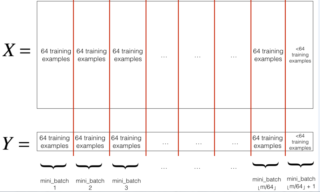
Exercise: Implement random_mini_batches. We coded the shuffling part for you. To help you with the partitioning step, we give you the following code that selects the indexes for the 1^st1and 2^nd mini-batches:

【中文翻译】

练习: 实施 random_mini_batches。我们为你编了洗牌的部分，为了帮助您执行分区步骤, 我们给出了以下代码, 它为1^st和 2^nd mini-batches 选择索引:

【code】

first_mini_batch_X = shuffled_X[:, 0 : mini_batch_size]
second_mini_batch_X = shuffled_X[:, mini_batch_size : 2 * mini_batch_size]
...

Note that the last mini-batch might end up smaller than mini_batch_size=64. Let ⌊s⌋ represents s rounded down to the nearest integer (this is math.floor(s) in Python). If the total number of examples is not a multiple of mini_batch_size=64 then there will bemini-batches with a full 64 examples, and the number of examples in the final mini-batch will be 

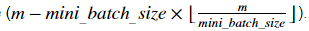
【中文翻译】

请注意, 最后的 mini-batch 可能会比 mini_batch_size=64 小。让⌊s⌋表示 s 四舍五入到最接近的整数 ( 在 Python 中的 math.floor(s) )。如果样本的总数不是 mini_batch_size=64 的倍数, 那么将有mini-batches有完整的64个样本, 最后 mini-batch 中的样本数将为

【code】

# GRADED FUNCTION: random_mini_batches

def random_mini_batches(X, Y, mini_batch_size = 64, seed = 0):
    """
    Creates a list of random minibatches from (X, Y)

    Arguments:
    X -- input data, of shape (input size, number of examples)
    Y -- true "label" vector (1 for blue dot / 0 for red dot), of shape (1, number of examples)
    mini_batch_size -- size of the mini-batches, integer

    Returns:
    mini_batches -- list of synchronous (mini_batch_X, mini_batch_Y) #同步列表 (mini_batch_X, mini_batch_Y)
    """

    np.random.seed(seed)            # To make your "random" minibatches the same as ours
    m = X.shape[1]                  # number of training examples   m=148
    mini_batches = []

    # Step 1: Shuffle (X, Y)
    permutation = list(np.random.permutation(m))
    shuffled_X = X[:, permutation]
    shuffled_Y = Y[:, permutation].reshape((1,m)) 

    # Step 2: Partition (shuffled_X, shuffled_Y). Minus the end case.
    num_complete_minibatches = math.floor(m/mini_batch_size) # number of mini batches of size mini_batch_size in your partitionning  =2
    for k in range(0, num_complete_minibatches):
        ### START CODE HERE ### (approx. 2 lines)
        mini_batch_X = shuffled_X[:, k * mini_batch_size : (k+1) * mini_batch_size]
        mini_batch_Y = shuffled_Y[:, k * mini_batch_size : (k+1) * mini_batch_size]
        ### END CODE HERE ###
        mini_batch = (mini_batch_X, mini_batch_Y)
        mini_batches.append(mini_batch)

    # Handling the end case (last mini-batch < mini_batch_size)
    if m % mini_batch_size != 0:
        ### START CODE HERE ### (approx. 2 lines)
        mini_batch_X = shuffled_X[:, mini_batch_size *  num_complete_minibatches : m]  # 64*2：148
        mini_batch_Y = shuffled_Y[:, mini_batch_size *  num_complete_minibatches : m]  #62*2：148
        ### END CODE HERE ###
        mini_batch = (mini_batch_X, mini_batch_Y)
        mini_batches.append(mini_batch)

    return mini_batches

X_assess, Y_assess, mini_batch_size = random_mini_batches_test_case()
mini_batches = random_mini_batches(X_assess, Y_assess, mini_batch_size)

print ("shape of the 1st mini_batch_X: " + str(mini_batches[0][0].shape))
print ("shape of the 2nd mini_batch_X: " + str(mini_batches[1][0].shape))
print ("shape of the 3rd mini_batch_X: " + str(mini_batches[2][0].shape))
print ("shape of the 1st mini_batch_Y: " + str(mini_batches[0][1].shape))
print ("shape of the 2nd mini_batch_Y: " + str(mini_batches[1][1].shape))
print ("shape of the 3rd mini_batch_Y: " + str(mini_batches[2][1].shape))
print ("mini batch sanity check: " + str(mini_batches[0][0][0][0:3])) #mini batch的 健全检查

【result】

shape of the 1st mini_batch_X: (12288, 64)
shape of the 2nd mini_batch_X: (12288, 64)
shape of the 3rd mini_batch_X: (12288, 20)
shape of the 1st mini_batch_Y: (1, 64)
shape of the 2nd mini_batch_Y: (1, 64)
shape of the 3rd mini_batch_Y: (1, 20)
mini batch sanity check: [ 0.90085595 -0.7612069   0.2344157 ]

Expected Output:

shape of the 1st mini_batch_X	(12288, 64)
shape of the 2nd mini_batch_X	(12288, 64)
shape of the 3rd mini_batch_X	(12288, 20)
shape of the 1st mini_batch_Y	(1, 64)
shape of the 2nd mini_batch_Y	(1, 64)
shape of the 3rd mini_batch_Y	(1, 20)
mini batch sanity check	[ 0.90085595 -0.7612069 0.2344157 ]

What you should remember:

• Shuffling and Partitioning are the two steps required to build mini-batches.
• Powers of two are often chosen to be the mini-batch size, e.g., 16, 32, 64, 128.

【中文翻译】

你应该记住的:

　　洗牌和分区是构建 mini-batches 所需的两个步骤。

　　2的幂通常被选择为 mini-batch 大小, 例如, 16、32、64、128。

3 - Momentum

Because mini-batch gradient descent makes a parameter update after seeing just a subset of examples, the direction of the update has some variance, and so the path taken by mini-batch gradient descent will "oscillate" toward convergence. Using momentum can reduce these oscillations.

Momentum takes into account the past gradients to smooth out the update. We will store the 'direction' of the previous gradients in the variable v. Formally, this will be the exponentially weighted average of the gradient on previous steps. You can also think of v as the "velocity" of a ball rolling downhill, building up speed (and momentum) according to the direction of the gradient/slope of the hill.

【中文翻译】

3-动量

由于 mini-batch 梯度下降只应用样本数据子集就进行参数更新, 因此更新的方向有一定的方差, 因此 mini-batch 梯度下降所采取的路径将 "振荡" 到收敛。使用动量可以减少这些振荡。 

动量考虑到过去的梯度来平滑更新。我们将在变量v中存储之前梯度的 "方向"。形式上, 这将是前面步骤的梯度的指数加权平均。你也可以认为v是球滚动下坡的 "速度", 根据山丘的梯度/斜坡，建立速度 (和动量) 的方向 。

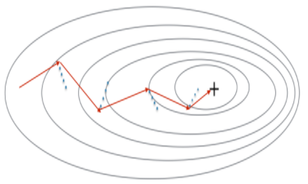
Figure 3: The red arrows shows the direction taken by one step of mini-batch gradient descent with momentum. The blue points show the direction of the gradient (with respect to the current mini-batch) on each step. Rather than just following the gradient, we let the gradient influence v and then take a step in the direction of v.

Exercise: Initialize the velocity. The velocity, v, is a python dictionary that needs to be initialized with arrays of zeros. Its keys are the same as those in the  grads dictionary, that is: for l=1,...,L

v["dW" + str(l+1)] = ... #(numpy array of zeros with the same shape as parameters["W" + str(l+1)])
v["db" + str(l+1)] = ... #(numpy array of zeros with the same shape as parameters["b" + str(l+1)])

Note that the iterator l starts at 0 in the for loop while the first parameters are v["dW1"] and v["db1"] (that's a "one" on the superscript). This is why we are shifting l to l+1 in the for loop.

【code】

# GRADED FUNCTION: initialize_velocity

def initialize_velocity(parameters):
    """
    Initializes the velocity as a python dictionary with:
                - keys: "dW1", "db1", ..., "dWL", "dbL"
                - values: numpy arrays of zeros of the same shape as the corresponding gradients/parameters.
    Arguments:
    parameters -- python dictionary containing your parameters.
                    parameters['W' + str(l)] = Wl
                    parameters['b' + str(l)] = bl

    Returns:
    v -- python dictionary containing the current velocity.
                    v['dW' + str(l)] = velocity of dWl
                    v['db' + str(l)] = velocity of dbl
    """

    L ) // 2 # number of layers in the neural networks  "//"表示返回整数
    v = {}= len(parameters

    # Initialize velocity
    for l in range(L):
        ### START CODE HERE ### (approx. 2 lines)
        v["dW" + str(l+1)] = np.zeros(( parameters['W' + str(l+1)].shape))
        v["db" + str(l+1)] =  np.zeros(( parameters['b' + str(l+1)].shape))
        ### END CODE HERE ###

    return v

parameters = initialize_velocity_test_case()

v = initialize_velocity(parameters)
print("v[\"dW1\"] = " + str(v["dW1"]))
print("v[\"db1\"] = " + str(v["db1"]))
print("v[\"dW2\"] = " + str(v["dW2"]))
print("v[\"db2\"] = " + str(v["db2"]))

【result】

v["dW1"] = [[ 0.  0.  0.]
 [ 0.  0.  0.]]
v["db1"] = [[ 0.]
 [ 0.]]
v["dW2"] = [[ 0.  0.  0.]
 [ 0.  0.  0.]
 [ 0.  0.  0.]]
v["db2"] = [[ 0.]
 [ 0.]
 [ 0.]]

Expected Output:

v["dW1"]	[[ 0. 0. 0.] [ 0. 0. 0.]]
v["db1"]	[[ 0.] [ 0.]]
v["dW2"]	[[ 0. 0. 0.] [ 0. 0. 0.] [ 0. 0. 0.]]
v["db2"]	[[ 0.] [ 0.] [ 0.]]

Exercise: Now, implement the parameters update with momentum. The momentum update rule is, for l=1,...,L：

where L is the number of layers, β is the momentum and α is the learning rate. All parameters should be stored in the parameters dictionary. Note that the iterator l starts at 0 in the for loop while the first parameters are W^[1] and b^[1](that's a "one" on the superscript). So you will need to shift l to l+1 when coding.

【code】

# GRADED FUNCTION: update_parameters_with_momentum

def update_parameters_with_momentum(parameters, grads, v, beta, learning_rate):
    """
    Update parameters using Momentum

    Arguments:
    parameters -- python dictionary containing your parameters:
                    parameters['W' + str(l)] = Wl
                    parameters['b' + str(l)] = bl
    grads -- python dictionary containing your gradients for each parameters:
                    grads['dW' + str(l)] = dWl
                    grads['db' + str(l)] = dbl
    v -- python dictionary containing the current velocity:
                    v['dW' + str(l)] = ...
                    v['db' + str(l)] = ...
    beta -- the momentum hyperparameter, scalar
    learning_rate -- the learning rate, scalar

    Returns:
    parameters -- python dictionary containing your updated parameters
    v -- python dictionary containing your updated velocities
    """

    L = len(parameters) // 2 # number of layers in the neural networks

    # Momentum update for each parameter
    for l in range(L):

        ### START CODE HERE ### (approx. 4 lines)
        # compute velocities
        v["dW" + str(l+1)] = beta *  v['dW' + str(l+1)]  + (1-beta) *  grads['dW' + str(l+1)]
        v["db" + str(l+1)] = beta *  v['db' + str(l+1)]  + (1-beta) *  grads['db' + str(l+1)]
        # update parameters
        parameters["W" + str(l+1)] =  parameters["W" + str(l+1)] - learning_rate *  v["dW" + str(l+1)]
        parameters["b" + str(l+1)] =  parameters["b" + str(l+1)] - learning_rate *  v["db" + str(l+1)]
        ### END CODE HERE ###

    return parameters, v

parameters, grads, v = update_parameters_with_momentum_test_case()

parameters, v = update_parameters_with_momentum(parameters, grads, v, beta = 0.9, learning_rate = 0.01)
print("W1 = " + str(parameters["W1"]))
print("b1 = " + str(parameters["b1"]))
print("W2 = " + str(parameters["W2"]))
print("b2 = " + str(parameters["b2"]))
print("v[\"dW1\"] = " + str(v["dW1"]))
print("v[\"db1\"] = " + str(v["db1"]))
print("v[\"dW2\"] = " + str(v["dW2"]))
print("v[\"db2\"] = " + str(v["db2"]))

【result】

W1 = [[ 1.62544598 -0.61290114 -0.52907334]
 [-1.07347112  0.86450677 -2.30085497]]
b1 = [[ 1.74493465]
 [-0.76027113]]
W2 = [[ 0.31930698 -0.24990073  1.4627996 ]
 [-2.05974396 -0.32173003 -0.38320915]
 [ 1.13444069 -1.0998786  -0.1713109 ]]
b2 = [[-0.87809283]
 [ 0.04055394]
 [ 0.58207317]]
v["dW1"] = [[-0.11006192  0.11447237  0.09015907]
 [ 0.05024943  0.09008559 -0.06837279]]
v["db1"] = [[-0.01228902]
 [-0.09357694]]
v["dW2"] = [[-0.02678881  0.05303555 -0.06916608]
 [-0.03967535 -0.06871727 -0.08452056]
 [-0.06712461 -0.00126646 -0.11173103]]
v["db2"] = [[ 0.02344157]
 [ 0.16598022]
 [ 0.07420442]]

Expected Output:

W1	[[ 1.62544598 -0.61290114 -0.52907334] [-1.07347112 0.86450677 -2.30085497]]
b1	[[ 1.74493465] [-0.76027113]]
W2	[[ 0.31930698 -0.24990073 1.4627996 ] [-2.05974396 -0.32173003 -0.38320915] [ 1.13444069 -1.0998786 -0.1713109 ]]
b2	[[-0.87809283] [ 0.04055394] [ 0.58207317]]
v["dW1"]	[[-0.11006192 0.11447237 0.09015907] [ 0.05024943 0.09008559 -0.06837279]]
v["db1"]	[[-0.01228902] [-0.09357694]]
v["dW2"]	[[-0.02678881 0.05303555 -0.06916608] [-0.03967535 -0.06871727 -0.08452056] [-0.06712461 -0.00126646 -0.11173103]]
v["db2"]	[[ 0.02344157] [ 0.16598022] [ 0.07420442]]

Note that:

• The velocity is initialized with zeros. So the algorithm will take a few iterations to "build up" velocity and start to take bigger steps.
• If β=0, then this just becomes standard gradient descent without momentum.

How do you choose β?

• The larger the momentum β  is, the smoother the update because the more we take the past gradients into account. But if β is too big, it could also smooth out the updates too much.
• Common values for β range from 0.8 to 0.999. If you don't feel inclined to tune this(如果你不倾向于调整这个), β=0.9 is often a reasonable default.
• Tuning the optimal β for your model might need trying several values to see what works best in term of reducing the value of the cost function J.

What you should remember:

• Momentum takes past gradients into account to smooth out the steps of gradient descent. It can be applied with batch gradient descent, mini-batch gradient descent or stochastic gradient descent.
• You have to tune a momentum hyperparameter β and a learning rate α.

4 - Adam

Adam is one of the most effective optimization algorithms for training neural networks. It combines ideas from RMSProp (described in lecture) and Momentum.

How does Adam work?

1. It calculates an exponentially weighted average of past gradients, and stores it in variables v (before bias correction) and v^corrected (with bias correction).
2. It calculates an exponentially weighted average of the squares of the past gradients, and stores it in variables s (before bias correction) and s^corrected(with bias correction).
3. It updates parameters in a direction based on combining information from "1" and "2".

The update rule is, for l=1,...,L:

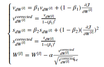
where:

• t counts the number of steps taken of Adam
• l is the number of layers
• β₁ and β₂ are hyperparameters that control the two exponentially weighted averages.
• α is the learning rate
• ε is a very small number to avoid dividing by zero

As usual, we will store all parameters in the parameters dictionary

Exercise: Initialize the Adam variables v,s which keep track of the past information.

Instruction: The variables v,s are python dictionaries that need to be initialized with arrays of zeros. Their keys are the same as for grads, that is: for l=1,...,L：

v["dW" + str(l+1)] = ... #(numpy array of zeros with the same shape as parameters["W" + str(l+1)])
v["db" + str(l+1)] = ... #(numpy array of zeros with the same shape as parameters["b" + str(l+1)])
s["dW" + str(l+1)] = ... #(numpy array of zeros with the same shape as parameters["W" + str(l+1)])
s["db" + str(l+1)] = ... #(numpy array of zeros with the same shape as parameters["b" + str(l+1)])

【code】

# GRADED FUNCTION: initialize_adam

def initialize_adam(parameters) :
    """
    Initializes v and s as two python dictionaries with:
                - keys: "dW1", "db1", ..., "dWL", "dbL"
                - values: numpy arrays of zeros of the same shape as the corresponding gradients/parameters.

    Arguments:
    parameters -- python dictionary containing your parameters.
                    parameters["W" + str(l)] = Wl
                    parameters["b" + str(l)] = bl

    Returns:
    v -- python dictionary that will contain the exponentially weighted average of the gradient.
                    v["dW" + str(l)] = ...
                    v["db" + str(l)] = ...
    s -- python dictionary that will contain the exponentially weighted average of the squared gradient.
                    s["dW" + str(l)] = ...
                    s["db" + str(l)] = ...

    """

    L = len(parameters) // 2 # number of layers in the neural networks
    v = {}
    s = {}

    # Initialize v, s. Input: "parameters". Outputs: "v, s".
    for l in range(L):
    ### START CODE HERE ### (approx. 4 lines)
        v["dW" + str(l+1)] = np.zeros(( parameters["W" + str(l+1)].shape))
        v["db" + str(l+1)] = np.zeros(( parameters["b" + str(l+1)].shape))
        s["dW" + str(l+1)] = np.zeros(( parameters["W" + str(l+1)].shape))
        s["db" + str(l+1)] = np.zeros(( parameters["b" + str(l+1)].shape))
    ### END CODE HERE ###

    return v, s

parameters = initialize_adam_test_case()

v, s = initialize_adam(parameters)
print("v[\"dW1\"] = " + str(v["dW1"]))
print("v[\"db1\"] = " + str(v["db1"]))
print("v[\"dW2\"] = " + str(v["dW2"]))
print("v[\"db2\"] = " + str(v["db2"]))
print("s[\"dW1\"] = " + str(s["dW1"]))
print("s[\"db1\"] = " + str(s["db1"]))
print("s[\"dW2\"] = " + str(s["dW2"]))
print("s[\"db2\"] = " + str(s["db2"]))

【result】

v["dW1"] = [[ 0.  0.  0.]
 [ 0.  0.  0.]]
v["db1"] = [[ 0.]
 [ 0.]]
v["dW2"] = [[ 0.  0.  0.]
 [ 0.  0.  0.]
 [ 0.  0.  0.]]
v["db2"] = [[ 0.]
 [ 0.]
 [ 0.]]
s["dW1"] = [[ 0.  0.  0.]
 [ 0.  0.  0.]]
s["db1"] = [[ 0.]
 [ 0.]]
s["dW2"] = [[ 0.  0.  0.]
 [ 0.  0.  0.]
 [ 0.  0.  0.]]
s["db2"] = [[ 0.]
 [ 0.]
 [ 0.]]

Expected Output:

v["dW1"]	[[ 0. 0. 0.] [ 0. 0. 0.]]
v["db1"]	[[ 0.] [ 0.]]
v["dW2"]	[[ 0. 0. 0.] [ 0. 0. 0.] [ 0. 0. 0.]]
v["db2"]	[[ 0.] [ 0.] [ 0.]]
s["dW1"]	[[ 0. 0. 0.] [ 0. 0. 0.]]
s["db1"]	[[ 0.] [ 0.]]
s["dW2"]	[[ 0. 0. 0.] [ 0. 0. 0.] [ 0. 0. 0.]]
s["db2"]	[[ 0.] [ 0.] [ 0.]]

 Exercise: Now, implement the parameters update with Adam. Recall the general update rule is, for l=1,...,L:

Note that the iterator l starts at 0 in the for loop while the first parameters are W^[1] and b^[1]. You need to shift l to l+1 when coding.

【code】

# GRADED FUNCTION: update_parameters_with_adam

def update_parameters_with_adam(parameters, grads, v, s, t, learning_rate = 0.01,
                                beta1 = 0.9, beta2 = 0.999,  epsilon = 1e-8):
    """
    Update parameters using Adam

    Arguments:
    parameters -- python dictionary containing your parameters:
                    parameters['W' + str(l)] = Wl
                    parameters['b' + str(l)] = bl
    grads -- python dictionary containing your gradients for each parameters:
                    grads['dW' + str(l)] = dWl
                    grads['db' + str(l)] = dbl
    v -- Adam variable, moving average of the first gradient, python dictionary
    s -- Adam variable, moving average of the squared gradient, python dictionary
    learning_rate -- the learning rate, scalar.
    beta1 -- Exponential decay hyperparameter for the first moment estimates
    beta2 -- Exponential decay hyperparameter for the second moment estimates
    epsilon -- hyperparameter preventing division by zero in Adam updates

    Returns:
    parameters -- python dictionary containing your updated parameters
    v -- Adam variable, moving average of the first gradient, python dictionary
    s -- Adam variable, moving average of the squared gradient, python dictionary
    """

    L = len(parameters) // 2                 # number of layers in the neural networks
    v_corrected = {}                         # Initializing first moment estimate, python dictionary
    s_corrected = {}                         # Initializing second moment estimate, python dictionary

    # Perform Adam update on all parameters
    for l in range(L):
        # Moving average of the gradients. Inputs: "v, grads, beta1". Output: "v".
        ### START CODE HERE ### (approx. 2 lines)
        v["dW" + str(l+1)] = beta1 *  v['dW' + str(l+1)]  + (1-beta1) *  grads['dW' + str(l+1)]
        v["db" + str(l+1)] = beta1 *  v['db' + str(l+1)]  + (1-beta1) *  grads['db' + str(l+1)]
        ### END CODE HERE ###

        # Compute bias-corrected first moment estimate. Inputs: "v, beta1, t". Output: "v_corrected".
        ### START CODE HERE ### (approx. 2 lines)
        v_corrected["dW" + str(l+1)] =  v["dW" + str(l+1)] / (1-beta1**t)
        v_corrected["db" + str(l+1)] = v["db" + str(l+1)] / (1-beta1**t)
        ### END CODE HERE ###

        # Moving average of the squared gradients. Inputs: "s, grads, beta2". Output: "s".
        ### START CODE HERE ### (approx. 2 lines)
        s["dW" + str(l+1)] =  beta2 *  s['dW' + str(l+1)]  + (1-beta2) *  (grads['dW' + str(l+1)]**2)
        s["db" + str(l+1)] =  beta2 *  s['db' + str(l+1)]  + (1-beta2) *  (grads['db' + str(l+1)]**2)
        ### END CODE HERE ###

        # Compute bias-corrected second raw moment estimate. Inputs: "s, beta2, t". Output: "s_corrected".
        ### START CODE HERE ### (approx. 2 lines)
        s_corrected["dW" + str(l+1)] =  s["dW" + str(l+1)] / (1-beta2**t)
        s_corrected["db" + str(l+1)] =  s["db" + str(l+1)] / (1-beta2**t)
        ### END CODE HERE ###

        # Update parameters. Inputs: "parameters, learning_rate, v_corrected, s_corrected, epsilon". Output: "parameters".
        ### START CODE HERE ### (approx. 2 lines)
        parameters["W" + str(l+1)] =  parameters["W" + str(l+1)] -  learning_rate *  v_corrected["dW" + str(l+1)] / (np.sqrt(s_corrected["dW" + str(l+1)]+  epsilon) )
        parameters["b" + str(l+1)] =  parameters["b" + str(l+1)] -  learning_rate *  v_corrected["db" + str(l+1)] / (np.sqrt(s_corrected["db" + str(l+1)]+  epsilon) )
        ### END CODE HERE ###

    return parameters, v, s

parameters, grads, v, s = update_parameters_with_adam_test_case()
parameters, v, s  = update_parameters_with_adam(parameters, grads, v, s, t = 2)

print("W1 = " + str(parameters["W1"]))
print("b1 = " + str(parameters["b1"]))
print("W2 = " + str(parameters["W2"]))
print("b2 = " + str(parameters["b2"]))
print("v[\"dW1\"] = " + str(v["dW1"]))
print("v[\"db1\"] = " + str(v["db1"]))
print("v[\"dW2\"] = " + str(v["dW2"]))
print("v[\"db2\"] = " + str(v["db2"]))
print("s[\"dW1\"] = " + str(s["dW1"]))
print("s[\"db1\"] = " + str(s["db1"]))
print("s[\"dW2\"] = " + str(s["dW2"]))
print("s[\"db2\"] = " + str(s["db2"]))

【result】

W1 = [[ 1.63178673 -0.61919778 -0.53561312]
 [-1.08040999  0.85796626 -2.29409733]]
b1 = [[ 1.75225313]
 [-0.75376553]]
W2 = [[ 0.32648046 -0.25681174  1.46954931]
 [-2.05269934 -0.31497584 -0.37661299]
 [ 1.14121081 -1.09245036 -0.16498684]]
b2 = [[-0.88529978]
 [ 0.03477238]
 [ 0.57537385]]
v["dW1"] = [[-0.11006192  0.11447237  0.09015907]
 [ 0.05024943  0.09008559 -0.06837279]]
v["db1"] = [[-0.01228902]
 [-0.09357694]]
v["dW2"] = [[-0.02678881  0.05303555 -0.06916608]
 [-0.03967535 -0.06871727 -0.08452056]
 [-0.06712461 -0.00126646 -0.11173103]]
v["db2"] = [[ 0.02344157]
 [ 0.16598022]
 [ 0.07420442]]
s["dW1"] = [[ 0.00121136  0.00131039  0.00081287]
 [ 0.0002525   0.00081154  0.00046748]]
s["db1"] = [[  1.51020075e-05]
 [  8.75664434e-04]]
s["dW2"] = [[  7.17640232e-05   2.81276921e-04   4.78394595e-04]
 [  1.57413361e-04   4.72206320e-04   7.14372576e-04]
 [  4.50571368e-04   1.60392066e-07   1.24838242e-03]]
s["db2"] = [[  5.49507194e-05]
 [  2.75494327e-03]
 [  5.50629536e-04]]

Expected Output:

W1	[[ 1.63178673 -0.61919778 -0.53561312] [-1.08040999 0.85796626 -2.29409733]]
b1	[[ 1.75225313] [-0.75376553]]
W2	[[ 0.32648046 -0.25681174 1.46954931] [-2.05269934 -0.31497584 -0.37661299] [ 1.14121081 -1.09245036 -0.16498684]]
b2	[[-0.88529978] [ 0.03477238] [ 0.57537385]]
v["dW1"]	[[-0.11006192 0.11447237 0.09015907] [ 0.05024943 0.09008559 -0.06837279]]
v["db1"]	[[-0.01228902] [-0.09357694]]
v["dW2"]	[[-0.02678881 0.05303555 -0.06916608] [-0.03967535 -0.06871727 -0.08452056] [-0.06712461 -0.00126646 -0.11173103]]
v["db2"]	[[ 0.02344157] [ 0.16598022] [ 0.07420442]]
s["dW1"]	[[ 0.00121136 0.00131039 0.00081287] [ 0.0002525 0.00081154 0.00046748]]
s["db1"]	[[ 1.51020075e-05] [ 8.75664434e-04]]
s["dW2"]	[[ 7.17640232e-05 2.81276921e-04 4.78394595e-04] [ 1.57413361e-04 4.72206320e-04 7.14372576e-04] [ 4.50571368e-04 1.60392066e-07 1.24838242e-03]]
s["db2"]	[[ 5.49507194e-05] [ 2.75494327e-03] [ 5.50629536e-04]]

You now have three working optimization algorithms (mini-batch gradient descent, Momentum, Adam). Let's implement a model with each of these optimizers and observe the difference.

5 - Model with different optimization algorithms

Lets use the following "moons" dataset to test the different optimization methods. (The dataset is named "moons" because the data from each of the two classes looks a bit like a crescent-shaped(新月形的) moon.)

【code】

train_X, train_Y = load_dataset()

We have already implemented a 3-layer neural network. You will train it with:

• Mini-batch Gradient Descent: it will call your function:
  • update_parameters_with_gd()
• Mini-batch Momentum: it will call your functions:
  • initialize_velocity() and update_parameters_with_momentum()
• Mini-batch Adam: it will call your functions:
  • initialize_adam() and update_parameters_with_adam()

【code】

def model(X, Y, layers_dims, optimizer, learning_rate = 0.0007, mini_batch_size = 64, beta = 0.9,
          beta1 = 0.9, beta2 = 0.999,  epsilon = 1e-8, num_epochs = 10000, print_cost = True):
    """
    3-layer neural network model which can be run in different optimizer modes.

    Arguments:
    X -- input data, of shape (2, number of examples)
    Y -- true "label" vector (1 for blue dot / 0 for red dot), of shape (1, number of examples)
    layers_dims -- python list, containing the size of each layer
    learning_rate -- the learning rate, scalar.
    mini_batch_size -- the size of a mini batch
    beta -- Momentum hyperparameter
    beta1 -- Exponential decay hyperparameter for the past gradients estimates
    beta2 -- Exponential decay hyperparameter for the past squared gradients estimates
    epsilon -- hyperparameter preventing division by zero in Adam updates
    num_epochs -- number of epochs
    print_cost -- True to print the cost every 1000 epochs

    Returns:
    parameters -- python dictionary containing your updated parameters
    """

    L = len(layers_dims)             # number of layers in the neural networks
    costs = []                       # to keep track of the cost
    t = 0                            # initializing the counter required for Adam update
    seed = 10                        # For grading purposes, so that your "random" minibatches are the same as ours

    # Initialize parameters
    parameters = initialize_parameters(layers_dims)

    # Initialize the optimizer
    if optimizer == "gd":
        pass # no initialization required for gradient descent
    elif optimizer == "momentum":
        v = initialize_velocity(parameters)
    elif optimizer == "adam":
        v, s = initialize_adam(parameters)

    # Optimization loop
    for i in range(num_epochs):

        # Define the random minibatches. We increment（增加） the seed to reshuffle（重新洗牌） differently the dataset after each epoch
        seed = seed + 1
        minibatches = random_mini_batches(X, Y, mini_batch_size, seed)

        for minibatch in minibatches:

            # Select a minibatch
            (minibatch_X, minibatch_Y) = minibatch

            # Forward propagation
            a3, caches = forward_propagation(minibatch_X, parameters)

            # Compute cost
            cost = compute_cost(a3, minibatch_Y)

            # Backward propagation
            grads = backward_propagation(minibatch_X, minibatch_Y, caches)

            # Update parameters
            if optimizer == "gd":
                parameters = update_parameters_with_gd(parameters, grads, learning_rate)
            elif optimizer == "momentum":
                parameters, v = update_parameters_with_momentum(parameters, grads, v, beta, learning_rate)
            elif optimizer == "adam":
                t = t + 1 # Adam counter
                parameters, v, s = update_parameters_with_adam(parameters, grads, v, s,
                                                               t, learning_rate, beta1, beta2,  epsilon)

        # Print the cost every 1000 epoch
        if print_cost and i % 1000 == 0:
            print ("Cost after epoch %i: %f" %(i, cost))
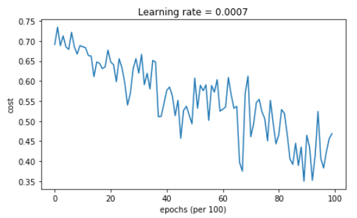
        if print_cost and i % 100 == 0:
            costs.append(cost)

    # plot the cost
    plt.plot(costs)
    plt.ylabel('cost')
    plt.xlabel('epochs (per 100)')
    plt.title("Learning rate = " + str(learning_rate))
    plt.show()

    return parameters

You will now run this 3 layer neural network with each of the 3 optimization methods.

5.1 - Mini-batch Gradient descent

Run the following code to see how the model does with mini-batch gradient descent.

【code】

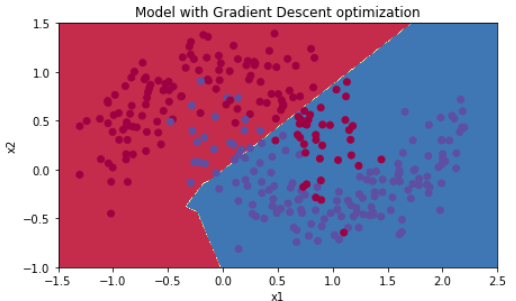
# train 3-layer model
layers_dims = [train_X.shape[0], 5, 2, 1]
parameters = model(train_X, train_Y, layers_dims, optimizer = "gd")

# Predict
predictions = predict(train_X, train_Y, parameters)

# Plot decision boundary
plt.title("Model with Gradient Descent optimization")
axes = plt.gca()
axes.set_xlim([-1.5,2.5])
axes.set_ylim([-1,1.5])
plot_decision_boundary(lambda x: predict_dec(parameters, x.T), train_X, train_Y)

【result】

Cost after epoch 0: 0.690736
Cost after epoch 1000: 0.685273
Cost after epoch 2000: 0.647072
Cost after epoch 3000: 0.619525
Cost after epoch 4000: 0.576584
Cost after epoch 5000: 0.607243
Cost after epoch 6000: 0.529403
Cost after epoch 7000: 0.460768
Cost after epoch 8000: 0.465586
Cost after epoch 9000: 0.464518

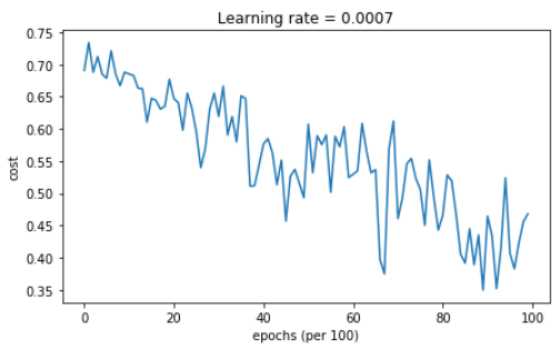
Accuracy: 0.796666666667

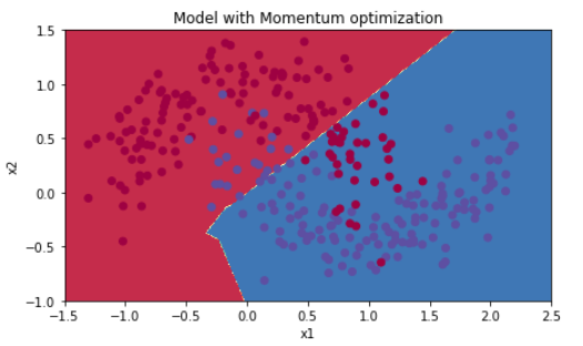
5.2 - Mini-batch gradient descent with momentum

Run the following code to see how the model does with momentum. Because this example is relatively simple, the gains from using momemtum are small; but for more complex problems you might see bigger gains.

【code】

# train 3-layer model
layers_dims = [train_X.shape[0], 5, 2, 1]
parameters = model(train_X, train_Y, layers_dims, beta = 0.9, optimizer = "momentum")

# Predict
predictions = predict(train_X, train_Y, parameters)

# Plot decision boundary
plt.title("Model with Momentum optimization")
axes = plt.gca()
axes.set_xlim([-1.5,2.5])
axes.set_ylim([-1,1.5])
plot_decision_boundary(lambda x: predict_dec(parameters, x.T), train_X, train_Y)

【result】

Cost after epoch 0: 0.690741
Cost after epoch 1000: 0.685341
Cost after epoch 2000: 0.647145
Cost after epoch 3000: 0.619594
Cost after epoch 4000: 0.576665
Cost after epoch 5000: 0.607324
Cost after epoch 6000: 0.529476
Cost after epoch 7000: 0.460936
Cost after epoch 8000: 0.465780
Cost after epoch 9000: 0.464740

Accuracy: 0.796666666667

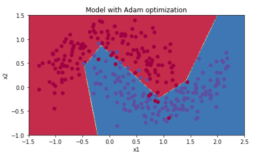
5.3 - Mini-batch with Adam mode

Run the following code to see how the model does with Adam.

【code】

# train 3-layer model
layers_dims = [train_X.shape[0], 5, 2, 1]
parameters = model(train_X, train_Y, layers_dims, optimizer = "adam")

# Predict
predictions = predict(train_X, train_Y, parameters)

# Plot decision boundary
plt.title("Model with Adam optimization")
axes = plt.gca()
axes.set_xlim([-1.5,2.5])
axes.set_ylim([-1,1.5])
plot_decision_boundary(lambda x: predict_dec(parameters, x.T), train_X, train_Y)

【reuslt】

Cost after epoch 0: 0.690552
Cost after epoch 1000: 0.185501
Cost after epoch 2000: 0.150830
Cost after epoch 3000: 0.074454
Cost after epoch 4000: 0.125959
Cost after epoch 5000: 0.104344
Cost after epoch 6000: 0.100676
Cost after epoch 7000: 0.031652
Cost after epoch 8000: 0.111973
Cost after epoch 9000: 0.197940

Accuracy: 0.94

5.4 - Summary

optimization method	accuracy	cost shape
Gradient descent	79.7%	oscillations
Momentum	79.7%	oscillations
Adam	94%	smoother

Momentum usually helps, but given the small learning rate and the simplistic dataset, its impact is almost negligeable. Also, the huge oscillations you see in the cost come from the fact that some minibatches are more difficult thans others for the optimization algorithm.

Adam on the other hand, clearly outperforms mini-batch gradient descent and Momentum. If you run the model for more epochs on this simple dataset, all three methods will lead to very good results. However, you've seen that Adam converges a lot faster.

Some advantages of Adam include:

• Relatively low memory requirements (though higher than gradient descent and gradient descent with momentum)
• Usually works well even with little tuning of hyperparameters (except α)

 

【中文翻译】

动量通常是有帮助的, 但是考虑到小的学习速度和简单的数据集, 它的影响几乎可以忽略。此外, 您在成本函数中看到的巨大振荡，是由于对优化算法来说，某些 minibatches 更难收敛。

另一方面, Adam明显优于 mini-batch 梯度下降和动量。如果您在这个简单的数据集上对模型迭代更多次, 所有三方法都将带来非常好的结果。然而, 你已经看到Adam收敛得更快了。

Adam 的一些优点包括:

　　相对较低的内存要求 (虽然高于梯度下降和动量梯度下降)

　　调整少许参数 (除了α)，通常就能得到很好的结果。

References:

• Adam paper: https://arxiv.org/pdf/1412.6980.pdf