Generative Modeling by Estimating Gradients of the Data Distribution

目录

• 概
• 主要内容
  • Langevin dynamics
  • Score Matching
  • Denoising Score Matching
  • Noise Conditional Score Networks
    • Slow mixing of Langevin dynamics
    • 损失函数
    • Annealed Langevin dynamics
    • 细节
• 代码

Song Y. and Ermon S. Generative modeling by estimating gradients of the data distribution. In Advances in Neural Information Processing Systems (NIPS), 2019.

概

当前生成模型, 要么依赖对抗损失(GAN), 要么依赖替代损失(VAE), 本文提出了基于score matching 训练, 以及利用annealed Langevin dynamics推断的模型, 思想非常有趣.

主要内容

Langevin dynamics

对于分布\(p(x)\), 我们可以通过下列方式迭代生成

\[\tilde{x}_t = \tilde{x}_{t-1} + \frac{\epsilon}{2} \nabla_x \log p (\tilde{x}_{t-1}) + \sqrt{\epsilon} z_t,
\]

其中\(\tilde{x}_0 \sim \pi(x)\)来自一个先验分布, \(z_t \sim \mathcal{N}(0, I)\). 当步长\(\epsilon \rightarrow 0\)并且\(T \rightarrow +\infty\)的时候, \(\tilde{x}_T\)可以认为是从\(p(x)\)中采样的样本.

注: 一般的Langevin, dynamics还需要在每一次迭代后计算一个接受概率然后判断是否接受, 不过在实际中这一步往往可以省略.

Score Matching

通过上述的迭代可以发现, 我们只需要获得\(\nabla_x \log p(x)\)即可采样\(x\), 我们可以期望通过下面的方式, 通过一个网络\(s_{\theta}(x)\)来逼近\(\nabla_x \log p_{data}(x)\):

\[\min_{\theta} \: \frac{1}{2} \mathbb{E}_{p_{data}(x)} [\| s_{\theta} (x) - \nabla_x \log p_{data}(x) \|_2^2],
\]

但是在实际中, 先验\(\log p_{data}(x)\)也是未知的, 幸运的是上述公式等价于:

\[\min_{\theta} \: \mathbb{E}_{p_{data}(x)} [\mathrm{tr}(\nabla_x s_{\theta} (x)) + \frac{1}{2} \|s_{\theta}(x)\|_2^2].
\]

注: 见 score matching

Denoising Score Matching

一个共识是, 所获得的数据往往是一个低维流形, 即其内在的维度实际上很低. 所以\(\mathbb{E}_{p_{data}(x)}\)在实际中会出现高密度的区域估计得很好, 但是低密度得区域估计得非常差. Denosing Score Matching提高了一个较为鲁棒的替代方法:

\[\min_{\theta} \: \frac{1}{2} \mathbb{E}_{q_{\sigma}(\tilde{x}|x)p_{data}(x)} [\| s_{\theta} (\tilde{x}) - \nabla_x \log q_{\sigma}(\tilde{x}|x) \|_2^2].
\]

当优化得足够好的时候,

\[s_{\theta^*}(x) = \nabla_x \log q_{\sigma}(x), \: q_{\sigma}(\tilde{x}) := \int q_{\sigma}(\tilde{x}|x) p_{data}(x) \mathrm{d}x.
\]

实际中, 通常取\(q_{\sigma}(\tilde{x}|x) = \mathcal{N}(\tilde{x}|x, \sigma^2 I)\), 相当于在真实数据\(x\)上加了一个扰动, 当扰动足够小(\(\sigma\)足够小)的时候, \(q_{\sigma}(x) \approx p_{data}(x)\), 则\(s_{\theta^*}(x) \approx \nabla_x \log p_{data}(x)\).

注: 为啥期望部分要有\(p_{data}\)? 实际上上述目标和score matching依旧是等价的.

Noise Conditional Score Networks

Slow mixing of Langevin dynamics

假设\(p_{data}(x) = \pi p_1(x) + (1 - \pi)p_2(x)\), 且\(p_1, p_2\)的支撑集合是互斥的, 那么 \(\nabla_{x} \log p_{data}(x)\)要么为\(\nabla_{x} \log p_{1}(x)\)或者\(\nabla_{x} \log p_{2}(x)\), 与\(\pi\)没有丝毫关联, 这会导致训练的结果与\(\pi\)也没有关联. 在实际中, 若\(p_1, p_2\)近似互斥, 也会产生类似的情况:

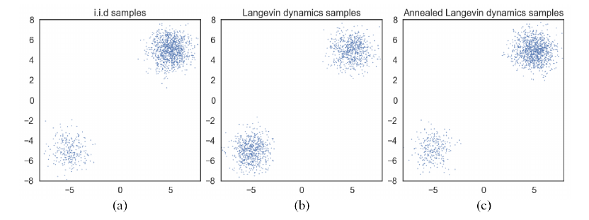
如上图所示, 通过Langevin dynamics采样的点几乎是1:1的, 这与真实的分布便有了出入.

作者的想法是, 设计一个noise conditional score networks:

\[s_\theta(x, \sigma),
\]

给定不同的\(\sigma\)其拟合不同扰动大小的\(p_{\sigma}\), 在采样中, 首先用大一点的\(\sigma\), 然后再逐步缩小, 这便是一种退火的思想. 显然, 一开始用大一点的\(\sigma\)能够为后面的采样提供更好更鲁棒的初始点.

损失函数

设定\(\sigma_i, i=1,2,\cdots, L\), 且满足:

\[\frac{\sigma_1}{\sigma_2} = \cdots = \frac{\sigma_{L-1}}{\sigma_L} > 1,
\]

即一个等比例(缩小)的数列.

对于每个\(\sigma\)采用如下损失:

\[\ell(\theta; \sigma) =
\frac{1}{2} \mathbb{E}_{p_{data}(x)} \mathbb{E}_{\mathcal{N}(\tilde{x}|x, \sigma I)} [\| s_{\theta} (\tilde{x}, \sigma) + \frac{\tilde{x} - x}{\sigma^2} \|_2^2].
\]

注: \(\nabla_{\tilde{x}} q_{\sigma}(\tilde{x}|x) = -\frac{\tilde{x} - x}{\sigma^2}\).

于是总损失为

\[\mathcal{L}(\theta; \{\sigma_i\}_{i=1}^L) := \frac{1}{L}\sum_{i=1}^L \lambda (\sigma_i)\ell(\theta;\sigma_i),
\]

\(\lambda(\sigma_i)\)为权重系数.

Annealed Langevin dynamics

Input: \(\{\sigma_i\}_{i=1}^L, \epsilon, T\);

1. 初始化\(x_0\);
2. For \(i=1,2,\cdots, L\) do:
   • \(\alpha_i \leftarrow \epsilon \cdot \sigma_i^2 / \sigma_L^2\);
   • For \(t=1,2,\cdots, T\) do:
     • 采样\(z_t \sim \mathcal{N}(0, I)\);
     • \(x_t \leftarrow x_{t-1} + \frac{\alpha_i}{2}s_{\theta}(x_{t-1}, \sigma) + \sqrt{\alpha_i} z_t\);
   • \(x_0 \leftarrow x_T\);

Output: \(x_T\).

细节

1. 关于参数\(\lambda(\sigma)\)的选择:
   
   作者推荐选择\(\lambda(\sigma) = \sigma^2\), 因为当优化到最优的时候, \(\|s_{\theta}(x, \sigma)\|_2 \propto 1 / \sigma\), 故\(\sigma^2 \ell(\theta;\sigma) = \frac{1}{2}\mathbb{E}[\|\sigma s_{\theta}(x, \sigma) + \frac{\tilde{x} - x}{\sigma} \|_2^2]\), 其中\(\sigma s_{\theta}(x, \sigma) \propto 1, \frac{\tilde{x} - x}{\sigma} \sim \mathcal{N}(0, I)\), 故\(\sigma^2 \ell_{\theta,\sigma}\)与\(\sigma\)无关.

2. 关于\(\alpha_i \leftarrow \epsilon \cdot \sigma_i^2 / \sigma_L^2\):

对于一次Langevin dynamic, 其获得的信息为: \(\frac{\alpha_i}{2} s_{\theta}(x_{t-1}, \sigma)\), 其噪声为\(\sqrt{\alpha_i}z_t\), 故其信噪比(signal-to-noise)为(应该是element-wise的计算?)

\[\frac{\alpha_i s_{\theta}(x, \sigma_i)}{2 \sqrt{\alpha_i} z},
\]

当我们按照算法中的取法时, 我们有

\[\begin{array}{ll}
\|\frac{\alpha_i s_{\theta}(x, \sigma_i)}{2 \sqrt{\alpha_i} z}\|_2^2
&\approx\frac{\alpha_i \| s_{\theta}(x, \sigma_i)\|_2^2}{4} \\
&\propto\frac{\|\sigma_i s_{\theta}(x, \sigma_i)\|_2^2}{4} \\
&\propto \frac{1}{4}.
\end{array}
\]

故采用此策略能够保证SNR保持一个稳定的值.

代码

原文代码