UNDERSTANDING THE GAUSSIAN DISTRIBUTION

Randomness is so present in our reality that we are used to take it for granted. Most of the phenomena which surround us have been generated by random processes. Hence, our brain is very good at recognise these random patterns. And is even better at spotting phenomena that should be random but they are actually aren’t. And this is when problems arise. Most software such as Unity or GameMaker simply lack the tools to generate realistic random numbers. This tutorial will introduce the Gaussian distribution, which plays a fundamental role in statistics since it is at the heart of many random phenomena in our everyday life.

Introduction

Let’s imagine you want to generate some random points on a plane. They can be enemies, trees, or whichever other entity you might thing of. The easiest way to do it in Unity is:

Vector3 position = new Vector3();

position.x = Random.Range(min,max),

position.y = Random.Range(min,max);

transform.position = position;

Using Random.Range will produce points distributed like in the blue box below. Some points might be closer than others, but globally they are all spread all over the place with the same density. We find approximately as many points on the left as there are on the right.

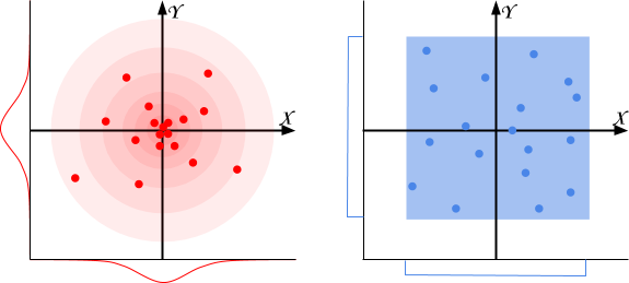
Many natural behaviours don’t follow this distribution. They are, instead, similar to the diagram on the left: these phenomena are Gaussian distributed. Thumb rule: when you have a natural phenomenon which should be around a certain value, the Gaussian distribution could be the way to go. For instance:

Damage: the amount of damage an enemy or a weapon inflicts;
Particle density: the amount of particles (sparkles, dust, …) around a particular object;
Grass and trees: how grass and trees are distributed in a biome; for instance, the position of plants near a lake, or the scatter or rocks around a mountain;
Enemy generation: if you want to generate enemies with random stats, you can design an “average” enemy and use the Gaussian distribution to get natural variations out of it.

This tutorial will explain what a Gaussian distribution exactly is, and why it appears in all the above mentioned phenomena.

Understanding uniform distributions

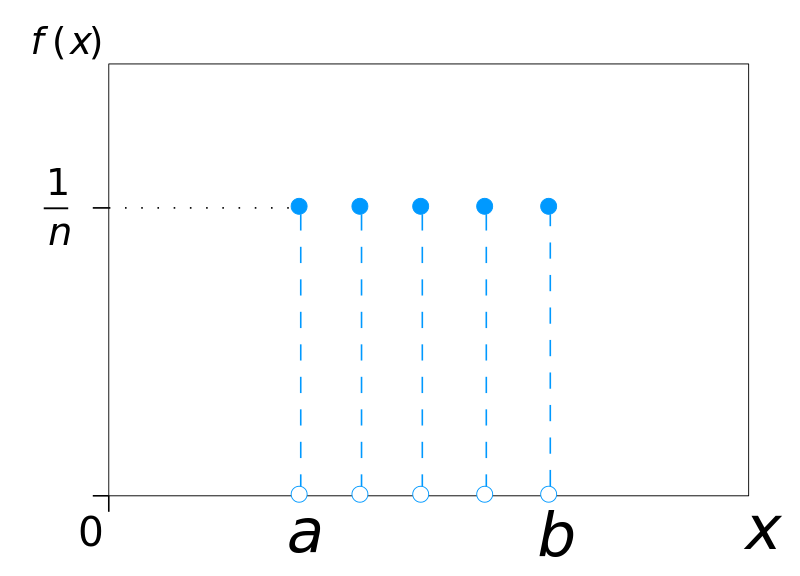
When you’re throwing a dice, there is one chance out of six to get a 6. Incidentally, every face of the dice also has the same chance. Statistically speaking, throwing a dice samples from a uniform discrete distribution (left). Every uniform distribution can be intuitively represented with a dice with faces. Each face has the same probability of being chosen . A function such as Random.Range, instead, returns values which are continuously uniformly distributed (right) over a particular range (typically, between 0 and 1).

In many cases, uniform distributions are a good choice. Choosing a random card from a deck, for instance, can be modelled perfectly with Random.Range.

What is a Gaussian distribution

There are other phenomena in the natural domain which don’t follow a uniform distribution. If you measure the height of all the people in a room, you’ll find that certain ranges occur more often than others. The majority of people will have a similar height, while extreme tall or short people are rare to find. If you randomly choose a person from that room, his height is likely to be close to the average height. These phenomena typically follow a distribution called the Gaussian (or normal) distribution. In a Gaussian distribution the probability of a given value to occur is given by:

If a uniform distribution is fully defined with its parameter , a Gaussian distribution is defined by two parameters and , namely the mean and the variance. The mean translates the curve left or right, centring it on the value which is expected to occur most frequently. The standard deviation, as the name suggests, indicates how easy is to deviate from the mean.

When a variable is generated by a phenomenon which is Gaussian distributed, it is usually indicated as:

Converging to a Gaussian distribution

Surprisingly enough, the equation for a Gaussian distribution can be derived from a uniform distribution. Despite looking quite different, they are deeply connected. Now let’s imagine a scenario in which a drunk man has to walk straight down a line. At every step, he has a 50% chance of moving left, and another 50% chance of moving right. Where is most likely to find the drunk man after 5 step? And after 100?

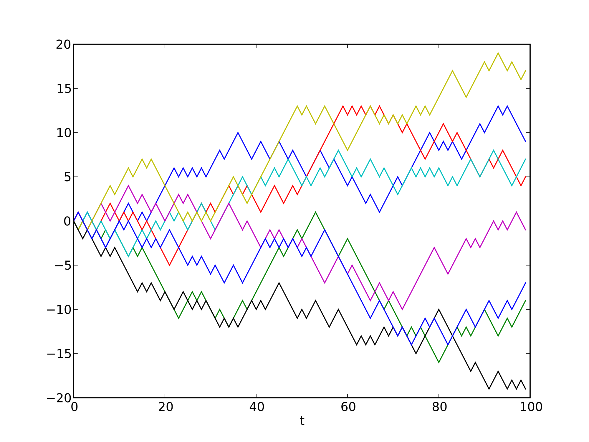
Since every step has the same probability, all of the above paths are equally likely to occur. Always going left is as likely as alternating left and right for the entire time. However, there is only one path which leads to his extreme left, while there are many more paths leading to the centre (more details here). For this reason, the drunk man is expected to stay closer to the centre. Having enough drunk men and enough time to walk, their final positions always approximate a Gaussian curve.

This concept can be explored without using actual drunk men. In the 19th century, Francis Galton came up with a device called bean machine: an old fashionedpachinko which allows for balls to naturally arrange themselves into the typical Gaussian bell.

This is related with the idea behind the central limit theorem; after a sufficiently large number of independent, well defined trials, results should approximate a Gaussian curve, regardless the underlying distribution of the original experiment.

Deriving the Gaussian distribution

If we look back at the bean machine, we can ask a very simple question: what is the probability for a ball to end up in a certain column? The answer depends on the number of right (or left) turns the ball makes. It is important to notice that the order doesn’t really matter: both (left, left, right) and (right, left, left) lead to the same column. And since there is a 50% change of going left or right at every turn, the question becomes: how many left turns is the ball making over iterations (in the example above: left turns over , iterations)? This can be calculated considering the chance of turning left times, with the chance of turning right times: . This form, however, accounts for only a single path: the one with left turns followed by right turns. We need to take into account all the possible permutations since they all lead to the same result. Without going too much into details, the number of permutations is described by the expression :

This is known as the binominal distribution and it answers the question of how likely is to obtain successes out of independent experiments, each one with the same probability .

Even so, it still doesn’t look very Gaussian at all. The idea is to bring to the infinity, switching from a discrete to a continuous distribution. In order to do that, we first need to expand the binomial coefficient using its factorial form:

then, factorial terms should be approximated using the Stirling’s formula:

The rest of the derivation is mostly mechanic and incredibly tedious; if you are interested, you can find it here. As a result we obtain:

with and .

Conclusion

This loosely explains why the majority of recurring, independent “natural” phenomena are, indeed, normally distributed. We are so surrounded by this distribution that our brain is incredibly good at recognise patterns which don’t follow it. This is the reason why, especially in games, is important to understand that some aspects must follow a normal distribution in order to be believable.

In the next post I’ll explore how to generate Gaussian distributed numbers, and how they can be used safely in your game.

Part 1: Understanding the Gaussian distribution
Part 2: How to generate Gaussian distributed numbers

Ways to Support

In the past months I've been dedicating more and more of my time to the creation of quality tutorials, mainly about game development and machine learning. If you think these posts have either helped or inspired you, please consider supporting me.