Sparse Autoencoder（一）

Neural Networks

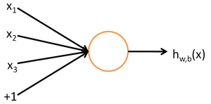
We will use the following diagram to denote a single neuron:

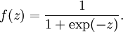
This "neuron" is a computational unit that takes as input x₁,x₂,x₃ (and a +1 intercept term), and outputs , where is called the activation function. In these notes, we will choose to be the sigmoid function:

Thus, our single neuron corresponds exactly to the input-output mapping defined by logistic regression.

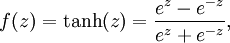
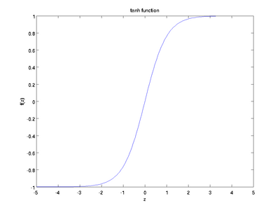
Although these notes will use the sigmoid function, it is worth noting that another common choice for f is the hyperbolic tangent, or tanh, function:

Here are plots of the sigmoid and tanh functions:

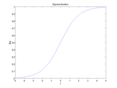
Finally, one identity that'll be useful later: If f(z) = 1 / (1 + exp( − z)) is the sigmoid function, then its derivative is given by f'(z) = f(z)(1 − f(z))

sigmoid 函数 或 tanh 函数都可用来完成非线性映射

Neural Network model

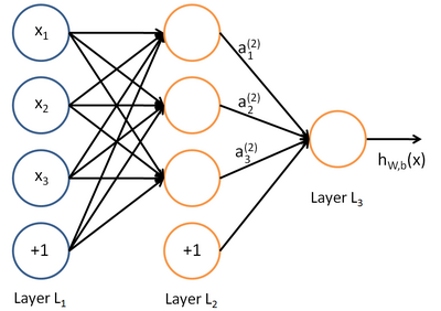
A neural network is put together by hooking together many of our simple "neurons," so that the output of a neuron can be the input of another. For example, here is a small neural network:

In this figure, we have used circles to also denote the inputs to the network. The circles labeled "+1" are called bias units, and correspond to the intercept term. The leftmost layer of the network is called the input layer, and the rightmost layer the output layer (which, in this example, has only one node). The middle layer of nodes is called the hidden layer, because its values are not observed in the training set. We also say that our example neural network has 3 input units (not counting the bias unit), 3 hidden units, and 1 output unit.

Our neural network has parameters (W,b) = (W⁽¹⁾,b⁽¹⁾,W⁽²⁾,b⁽²⁾), where we write to denote the parameter (or weight) associated with the connection between unit j in layer l, and unit i in layerl + 1. (Note the order of the indices.) Also, is the bias associated with unit i in layer l + 1.

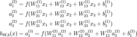
We will write to denote the activation (meaning output value) of unit i in layer l. For l = 1, we also use to denote the i-th input. Given a fixed setting of the parameters W,b, our neural network defines a hypothesis h_W,b(x) that outputs a real number. Specifically, the computation that this neural network represents is given by:

每层都是线性组合 + 非线性映射

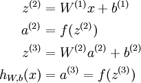
In the sequel, we also let denote the total weighted sum of inputs to unit i in layer l, including the bias term (e.g., ), so that .

Note that this easily lends itself to a more compact notation. Specifically, if we extend the activation function to apply to vectors in an element-wise fashion (i.e., f([z₁,z₂,z₃]) = [f(z₁),f(z₂),f(z₃)]), then we can write the equations above more compactly as:

We call this step forward propagation.

Backpropagation Algorithm

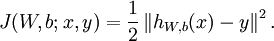
for a single training example (x,y), we define the cost function with respect to that single example to be:

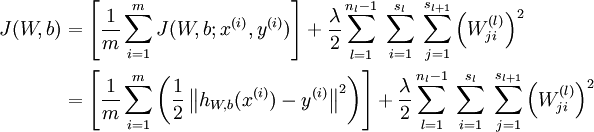
This is a (one-half) squared-error cost function. Given a training set of m examples, we then define the overall cost function to be:

J(W,b;x,y) is the squared error cost with respect to a single example; J(W,b) is the overall cost function, which includes the weight decay term.

Our goal is to minimize J(W,b) as a function of W and b. To train our neural network, we will initialize each parameter and each to a small random value near zero (say according to a Normal(0,ε²) distribution for some small ε, say 0.01), and then apply an optimization algorithm such as batch gradient descent.Finally, note that it is important to initialize the parameters randomly, rather than to all 0's. If all the parameters start off at identical values, then all the hidden layer units will end up learning the same function of the input (more formally, will be the same for all values of i, so that for any input x). The random initialization serves the purpose of symmetry breaking.

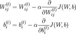
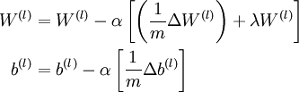
One iteration of gradient descent updates the parameters W,b as follows:

The two lines above differ slightly because weight decay is applied to W but not b.

The intuition behind the backpropagation algorithm is as follows. Given a training example (x,y), we will first run a "forward pass" to compute all the activations throughout the network, including the output value of the hypothesis h_W,b(x). Then, for each node i in layer l, we would like to compute an "error term" that measures how much that node was "responsible" for any errors in our output.

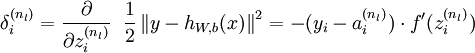
For an output node, we can directly measure the difference between the network's activation and the true target value, and use that to define (where layer n_l is the output layer). For hidden units, we will compute based on a weighted average of the error terms of the nodes that uses as an input. In detail, here is the backpropagation algorithm:

• 1，Perform a feedforward pass, computing the activations for layers L₂, L₃, and so on up to the output layer .

2，For each output unit i in layer n_l (the output layer), set

For

For each node i in layer l, set

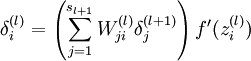
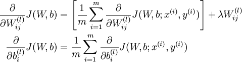
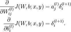
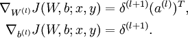
4，Compute the desired partial derivatives, which are given as:

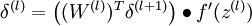
We will use "" to denote the element-wise product operator (denoted ".*" in Matlab or Octave, and also called the Hadamard product), so that if , then . Similar to how we extended the definition of to apply element-wise to vectors, we also do the same for (so that ).

The algorithm can then be written:

1. 1，Perform a feedforward pass, computing the activations for layers , , up to the output layer , using the equations defining the forward propagation steps

2，For the output layer (layer ), set

 

3，For

Set

 

4，Compute the desired partial derivatives:

 

Implementation note: In steps 2 and 3 above, we need to compute for each value of . Assuming is the sigmoid activation function, we would already have stored away from the forward pass through the network. Thus, using the expression that we worked out earlier for , we can compute this as .

Finally, we are ready to describe the full gradient descent algorithm. In the pseudo-code below, is a matrix (of the same dimension as ), and is a vector (of the same dimension as ). Note that in this notation, "" is a matrix, and in particular it isn't " times ." We implement one iteration of batch gradient descent as follows:

1. 1，Set , (matrix/vector of zeros) for all .
2. 2，For to ,
   1. Use backpropagation to compute and .
   2. Set .
   3. Set .
3. 3，Update the parameters: