OpenCV 之 平面单应性

上篇 OpenCV 之 图象几何变换 介绍了等距、相似和仿射变换，本篇侧重投影变换的平面单应性、OpenCV相关函数、应用实例等。

1  投影变换

1.1  平面单应性

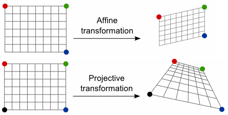
投影变换 (Projective Transformation)，是仿射变换的泛化 (或普遍化)，二者区别如下：

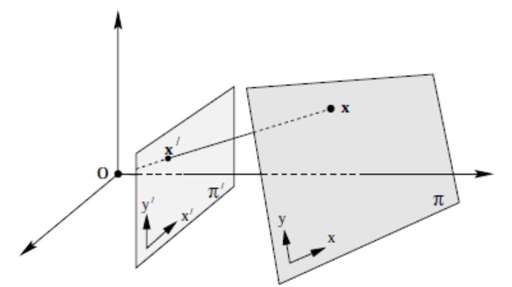
假定平面 $P^{2}$ 与 $Q^{2}$ 之间，存在映射 $H_{3 \times 3}$，使得 $P^{2}$ 内任意点 $(x_p, y_q, 1)$，满足下式：

$\quad \begin{bmatrix} x_q \\ y_q \\  1 \end{bmatrix} = \begin{bmatrix} h_{11} & h_{12} & h_{13} \\ h_{21} & h_{22} & h_{23} \\ h_{31} & h_{32} & h_{33} \end{bmatrix} \begin{bmatrix} x_p \\ y_p \\  1 \end{bmatrix}  =   H_{3 \times 3} \begin{bmatrix} x_p\\ y_p \\  1 \end{bmatrix}$

当 $H$ 非奇异时，$P^{2}$ 与 $Q^{2}$ 之间的映射即为 2D 投影变换，也称 平面单应性， $H_{3 \times 3}$ 则为 单应性矩阵

例如：在相机标定中，如果选取了 二维平面标定板，则 物平面 和 像平面 之间的映射，就是一种典型的 平面单应性

1.2  单应性矩阵

$H$ 有 9 个未知数，但实际只有 8 个自由度 (DoF)，其归一化通常有两种方法：

第一种方法，令 $h_{33}=1$；第二种方法，加单位向量限制  $h_{11}^2+h_{12}^2+h_{13}^2+h_{21}^2+h_{22}^2+h_{23}^2+h_{31}^2+h_{32}^2+h_{33}^2=1$

下面接着第一种方法，继续推导公式如下：

$\quad x' = \dfrac{h_{11}x + h_{12}y + h_{13}}{h_{31}x + h_{32}y + 1} $

$\quad y' = \dfrac{h_{21}x + h_{22}y + h_{23}}{h_{31}x + h_{32}y + 1} $

整理得：

$\quad x \cdot h_{11} + y \cdot h_{12} + h_{13} - xx' \cdot h_{31} - yx' \cdot h_{32} = x' $

$\quad x \cdot h_{21} + y \cdot h_{22} + h_{23} - xy' \cdot h_{31} - yy' \cdot h_{32} = y' $

一组对应特征点 $(x, y) $ -> $ (x', y')$ 可构造 2 个方程，要求解 8 个未知数 (归一化后的)，则需要 8 个方程，4 组对应特征点

$\quad \begin{bmatrix} x_{1} & y_{1} & 1 &0 &0&0 & -x_{1}x'_{1} & -y_{1}x'_{1} \\ 0&0&0& x_{1} & y_{1} &1& -x_{1}y'_{1} & -y_{1}y'_{1}  \\ x_{2} & y_{2} & 1 &0 &0&0 & -x_{2}x'_{2} & -y_{2}x'_{2} \\ 0&0&0& x_{2} & y_{2} &1& -x_{2}y'_{2} & -y_{2}y'_{2} \\ x_{3} & y_{3} & 1 &0 &0&0 & -x_{3}x'_{3} & -y_{3}x'_{3} \\ 0&0&0& x_{3} & y_{3} &1& -x_{3}y'_{3} & -y_{3}y'_{3}  \\ x_{4} & y_{4} & 1 &0 &0&0 & -x_{4}x'_{4} & -y_{4}x'_{4} \\ 0&0&0& x_{4} & y_{4} &1& -x_{4}y'_{4} & -y_{4}y'_{4} \end{bmatrix} \begin{bmatrix} h_{11} \\ h_{12}\\h_{13}\\h_{21}\\h_{22}\\h_{23}\\h_{31}\\h_{32} \end{bmatrix} = \begin{bmatrix} x'_{1}\\y'_{1}\\x'_{2}\\y'_{2}\\x'_{3}\\y'_{3}\\x'_{4}\\y'_{4}  \end{bmatrix} $

因此，求 $H$ 可转化为 $Ax=b$ 的通用解，参见 OpenCV 中 getPerspectiveTransform() 函数的源码实现

2  OpenCV 函数

2.1  投影变换矩阵

a)  四组对应特征点：已知四组对应特征点坐标，带入 getPerspectiveTransform() 函数中，可求解 src 投影到 dst 的单应性矩阵 $H_{3 \times 3}$

Mat getPerspectiveTransform (
    const Point2f     src[],    // 原图像的四角顶点坐标
    const Point2f     dst[],    // 目标图像的四角顶点坐标
    int solveMethod = DECOMP_LU // solve() 的解法
)

该函数的源代码实现如下：先构造8组方程，转化为 $Ax=b$ 的问题，调用 solve() 函数来求解

Mat getPerspectiveTransform(const Point2f src[], const Point2f dst[], int solveMethod)
{
    Mat M(3, 3, CV_64F), X(8, 1, CV_64F, M.ptr());
    double a[8][8], b[8];
    Mat A(8, 8, CV_64F, a), B(8, 1, CV_64F, b);

    for( int i = 0; i < 4; ++i )
    {
        a[i][0] = a[i+4][3] = src[i].x;
        a[i][1] = a[i+4][4] = src[i].y;
        a[i][2] = a[i+4][5] = 1;
        a[i][3] = a[i][4] = a[i][5] =
        a[i+4][0] = a[i+4][1] = a[i+4][2] = 0;
        a[i][6] = -src[i].x*dst[i].x;
        a[i][7] = -src[i].y*dst[i].x;
        a[i+4][6] = -src[i].x*dst[i].y;
        a[i+4][7] = -src[i].y*dst[i].y;
        b[i] = dst[i].x;
        b[i+4] = dst[i].y;
    }

    solve(A, B, X, solveMethod);
    M.ptr<double>()[8] = 1.;

    return M;
}

b)  多组对应特征点：对于两个平面之间的投影变换，只要求得对应的两组特征点，带入 findHomography() 函数，便可得到 srcPoints 投影到 dstPoints 的 $H_{3 \times 3}$

Mat findHomography (
    InputArray      srcPoints,   // 原始平面特征点坐标，类型是 CV_32FC2 或 vector<Point2f>
    InputArray      dstPoints,   // 目标平面特征点坐标，类型是 CV_32FC2 或 vector<Point2f>
    int method = 0,              // 0--最小二乘法; RANSAC--基于ransac的方法
    double ransacReprojThreshold = 3, // 最大允许反投影误差
    OutputArray mask = noArray(),     //
    const int maxIters = 2000,        // 最多迭代次数
    const double confidence = 0.995   // 置信水平
)

2.2  投影变换图像

已知单应性矩阵$H_{3 \times 3}$，将任意图像代入 warpPerspective() 中，便可得到经过 2D投影变换 的目标图像

void warpPerspective (
    InputArray      src,  // 输入图像
    OutputArray     dst,  // 输出图象(大小 dsize，类型同 src)
    InputArray        M,  // 3x3 单应性矩阵
    Size          dsize,  // 输出图像的大小
    int     flags = INTER_LINEAR,         // 插值方法
    int     borderMode = BORDER_CONSTANT, //
    const Scalar& borderValue = Scalar()  //
)                

3  单应性的应用

3.1  图像校正

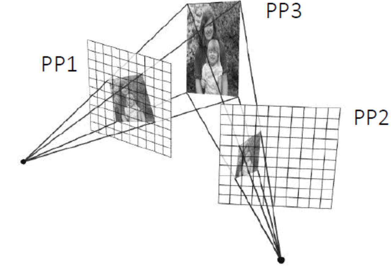
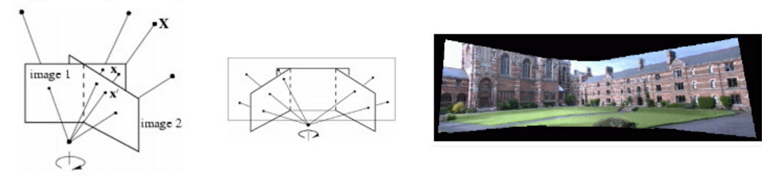
像平面 image1 和 image2 是相机在不同位置对同一物平面所成的像，分别对应右下图的 PP1、PP2 和 PP3，这三个平面任选两个都互有 平面单应性

      

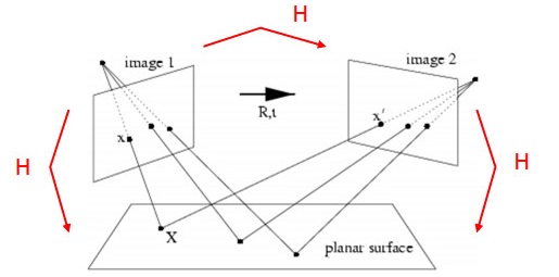
以相机标定过程为例，当相机从不同角度对标定板进行拍摄时，利用任意两个像平面之间的单应性，可将各角度拍摄的图像，转换为某一特定视角的图像

3.2  图像拼接

当相机围绕其投影轴，只做旋转运动时，所有的像素点可等效视为在一个无穷远的平面上，则单应性矩阵可由旋转变换 $R$ 和 相机标定矩阵 $K$ 来表示

$\quad \large s \begin{bmatrix} x' \\ y' \\1 \end{bmatrix} = \large K \cdot \large R \cdot \large K^{-1} \begin{bmatrix} x \\ y \\ 1 \end{bmatrix}$

因此，如果已知相机的标定矩阵，以及旋转变换前后的位姿，可利用平面单应性，将旋转变换前后的两幅图像拼接起来

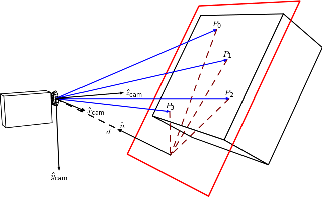
3.3  位姿估计

如下所示，当相机对着一个带多个特征点的平面拍摄时，物、像平面之间便有了单应性映射 $H_1$：定义 $\widehat{n}$ 为平面的法向量，$d$ 为物平面到相机的距离 (沿着$\widehat{n}$的方向)

如果相机变换位姿，从不同角度对该平面进行成像，则可建立起相机所有位姿和该平面的单应性映射 $H_2，H_3，H_4 ... $ ，从而计算得出相机的位姿 (也称 PnP 问题)

4  代码示例

4.1  图像校正

#include <iostream>

#include "opencv2/core.hpp"
#include "opencv2/imgproc.hpp"
#include "opencv2/highgui.hpp"
#include "opencv2/calib3d.hpp"

using namespace std;
using namespace cv;

Size kPatternSize = Size(9, 6);

int main()
{
    // 1) read image
    Mat src = imread("chessboard1.jpg");
    Mat dst = imread("chessboard2.jpg");
    if (src.empty() || dst.empty())
        return -1;

    // 2) find chessboard corners
    vector<Point2f> corners1, corners2;
    bool found1 = findChessboardCorners(src, kPatternSize, corners1);
    bool found2 = findChessboardCorners(dst, kPatternSize, corners2);
    if (!found1 || !found2)
        return -1;

    // 3) get subpixel accuracy of corners
    Mat src_gray, dst_gray;
    cvtColor(src, src_gray, COLOR_BGR2GRAY);
    cvtColor(dst, dst_gray, COLOR_BGR2GRAY);
    cornerSubPix(src_gray, corners1, Size(11, 11), Size(-1, -1), TermCriteria(TermCriteria::EPS | cv::TermCriteria::COUNT, 30, 0.1));
    cornerSubPix(dst_gray, corners2, Size(11, 11), Size(-1, -1), TermCriteria(TermCriteria::EPS | cv::TermCriteria::COUNT, 30, 0.1));

    // 4)
    Mat H = findHomography(corners1, corners2, RANSAC);
    // 5)
    Mat src_warp;
    warpPerspective(src, src_warp, H, src.size());

    // 6)
    imshow("src", src);
    imshow("dst", dst);
    imshow("src_warp", src_warp);

    waitKey(0);
}

结果如下：

    

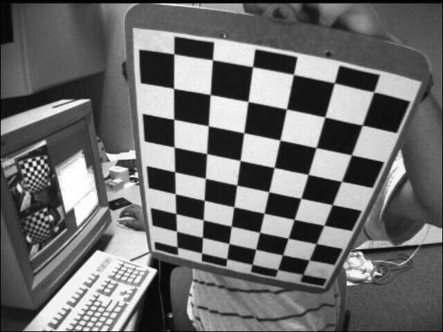
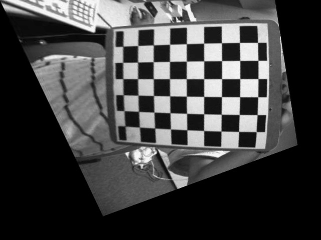
视角1的图像                                                           视角2的图像                                                视角1的图像校正为视角2

4.2  图像拼接

用 Blender 软件，获取相机只做旋转变换时的视图1和视图2，在已知相机标定矩阵和旋转矩阵的情况下，可计算出两个视图之间的单应性矩阵，从而完成拼接。

#include "opencv2/core.hpp"
#include "opencv2/imgproc.hpp"
#include "opencv2/highgui.hpp"
#include "opencv2/calib3d.hpp"

using namespace cv;

int main()
{
    // 1) read image
    Mat img1 = imread("view1.jpg");
    Mat img2 = imread("view2.jpg");
    if (img1.empty() || img2.empty())
        return -1;

    // 2) camera pose from Blender at location 1
    Mat c1Mo = (Mat_<double>(4, 4) << 0.9659258723258972, 0.2588190734386444, 0.0, 1.5529145002365112,
                                      0.08852133899927139, -0.3303661346435547, -0.9396926164627075, -0.10281121730804443,
                                      -0.24321036040782928, 0.9076734185218811, -0.342020183801651, 6.130080699920654,
                                      0, 0, 0, 1);

    // camera pose from Blender at location 2
    Mat c2Mo = (Mat_<double>(4, 4) << 0.9659258723258972, -0.2588190734386444, 0.0, -1.5529145002365112,
                                      -0.08852133899927139, -0.3303661346435547, -0.9396926164627075, -0.10281121730804443,
                                      0.24321036040782928, 0.9076734185218811, -0.342020183801651, 6.130080699920654,
                                      0, 0, 0, 1);

    // 3) camera intrinsic parameters
    Mat cameraMatrix = (Mat_<double>(3, 3) << 700.0, 0.0, 320.0,
                                              0.0, 700.0, 240.0,
                                              0, 0, 1);
    // 4) extract rotation
    Mat R1 = c1Mo(Range(0, 3), Range(0, 3));
    Mat R2 = c2Mo(Range(0, 3), Range(0, 3));

    // 5) compute rotation displacement: c1Mo * oMc2
    Mat R_2to1 = R1 * R2.t();

    // 6) homography
    Mat H = cameraMatrix * R_2to1 * cameraMatrix.inv();
    H /= H.at<double>(2, 2);

    // 7) warp
    Mat img_stitch;
    warpPerspective(img2, img_stitch, H, Size(img2.cols * 2, img2.rows));

    // 8) stitch
    Mat half = img_stitch(Rect(0, 0, img1.cols, img1.rows));
    img1.copyTo(half);
    imshow("Panorama stitching", img_stitch);

    waitKey(0);
}

输出结果如下：

     

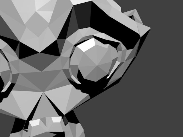
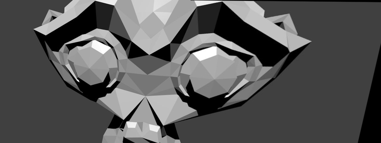
相机视图1                                              相机视图1                                                                                   拼接后的视图

4.3  相机位姿估计

一组从不同视角拍摄的标定板，预先知道其拍摄相机的内参，则调用 solvePnPRansac() 函数，可估计出该相机拍摄时的位姿

#include "opencv2/core.hpp"
#include "opencv2/imgproc.hpp"
#include "opencv2/highgui.hpp"
#include "opencv2/calib3d.hpp"

using namespace std;
using namespace cv;

Size kPatternSize = Size(9, 6);
float kSquareSize = 0.025;

int main()
{
    // 1) read image
    Mat src = imread("images/left01.jpg");
    if (src.empty())
        return -1;
    // prepare for subpixel corner
    Mat src_gray;
    cvtColor(src, src_gray, COLOR_BGR2GRAY);

    // 2) find chessboard corners
    vector<Point2f> corners;
    bool patternfound = findChessboardCorners(src, kPatternSize, corners);

    // 3) get subpixel accuracy
    if (patternfound) {
        cornerSubPix(src_gray, corners, Size(11, 11), Size(-1, -1), TermCriteria(TermCriteria::EPS + TermCriteria::MAX_ITER, 30, 0.1));
    } else {
        return -1;
    }

    // 4) define object coordinates
    vector<Point3f> objectPoints;
    for (int i = 0; i < kPatternSize.height; i++)
    {
        for (int j = 0; j < kPatternSize.width; j++)
        {
            objectPoints.push_back(Point3f(float(j*kSquareSize), float(i*kSquareSize), 0));
        }
    }

    // 5) input camera intrinsic parameters
    Mat cameraMatrix = (Mat_<double>(3, 3) << 5.3591573396163199e+02, 0.0, 3.4228315473308373e+02,
                                              0.0, 5.3591573396163199e+02, 2.3557082909788173e+02,
                                              0.0, 0.0, 1.);
    Mat distCoeffs = (Mat_<double>(5, 1) << -2.6637260909660682e-01, -3.8588898922304653e-02, 1.7831947042852964e-03,
                                            -2.8122100441115472e-04, 2.3839153080878486e-01);

    // 6) compute rotation and translation vectors
    Mat rvec, tvec;
    solvePnPRansac(objectPoints, corners, cameraMatrix, distCoeffs, rvec, tvec);

    // 7) project estimated pose on the image
    drawFrameAxes(src, cameraMatrix, distCoeffs, rvec, tvec, 2*kSquareSize);
    imshow("Pose from coplanar points", src);

    waitKey(0);
}

从不同角度拍摄的标定板，其估计的相机位姿如下：

          

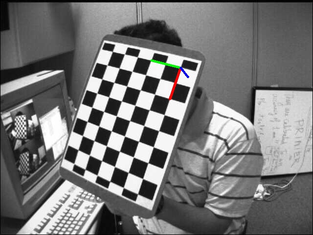
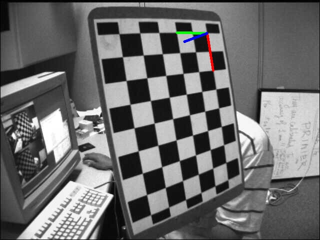
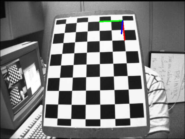
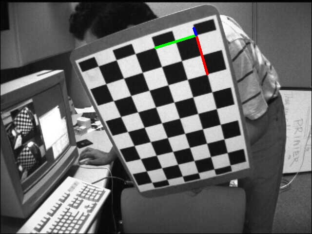
位姿1                                                                      位姿2                                                                               位姿3                                                               位姿4

参考资料：

OpenCV Tutorials / feature2d module / Basic concepts of the homography explained with code

OpenCV-Python Tutorials / Camera Calibration and 3D Reconstruction / Pose Estimation

Affine and Projective Transformations