matplotlib 进阶之Customizing Figure Layouts Using GridSpec and Other Functions

对Gridspec的一些精细的调整
利用SubplotSpec
- fig.add_grdispec; gs.subgridspec
一个利用Subplotspec的复杂例子
函数链接

matplotlib教程学习笔记

如何创建网格形式的axes的组合呢：

subplots()
GridSpec
SubplotSpec
subplot2grid()

import matplotlib

import matplotlib.pyplot as plt

import matplotlib.gridspec as gridspec

第一个例子是利用subplots()和gridspec来创建一个\(2\times 2\)的网格

首先利用subplots()是很容易做到这一点的：

fig1, fi_axes = plt.subplots(ncols=2, nrows=2, constrained_layout=True) #constrain_layout参数似乎是控制是否会重叠的

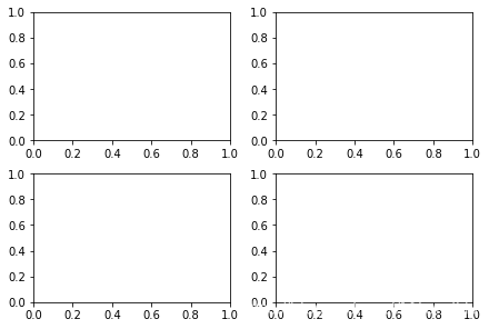
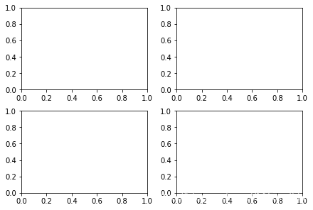
使用gridspec需要先创建一个fig对象，再创建Gridspec对象，然后将实例传入add_subplot()，gridspec的使用习惯和numpy数组是相当的

fig2 = plt.figure(constrained_layout=True)

spec2 = gridspec.GridSpec(ncols=2, nrows=2, figure=fig2)

f2_ax1 = fig2.add_subplot(spec2[0, 0])

f2_ax2 = fig2.add_subplot(spec2[0, 1])

f2_ax3 = fig2.add_subplot(spec2[1, 0])

f2_ax4 = fig2.add_subplot(spec2[1, 1])

gridspec有什么厉害的地方呢，我们可以通过索引和切片操作，使得某些axes占据多个格子

fig3 = plt.figure(constrained_layout=True)

gs = fig3.add_gridspec(3, 3)

f3_ax1 = fig3.add_subplot(gs[0, :])

f3_ax1.set_title('gs[0, :]')

f3_ax2 = fig3.add_subplot(gs[1, :-1])

f3_ax2.set_title('gs[1, :-1]')

f3_ax3 = fig3.add_subplot(gs[1:, -1])

f3_ax3.set_title('gs[1:, -1]')

f3_ax4 = fig3.add_subplot(gs[-1, 0])

f3_ax4.set_title('gs[-1, 0]')

f3_ax5 = fig3.add_subplot(gs[-1, -2])

f3_ax5.set_title('gs[-1, -2]');

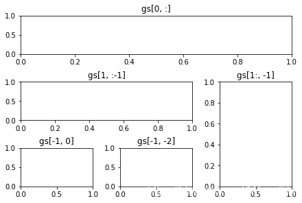
fig4 = plt.figure(constrained_layout=True)

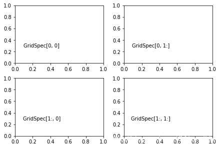
spec4 = fig4.add_gridspec(ncols=2, nrows=2)

anno_opts = dict(xy=(0.3, 0.3), xycoords='axes fraction',

                 va='center', ha='center')

f4_ax1 = fig4.add_subplot(spec4[0, 0])

f4_ax1.annotate('GridSpec[0, 0]', **anno_opts)

fig4.add_subplot(spec4[0, 1]).annotate('GridSpec[0, 1:]', **anno_opts)

fig4.add_subplot(spec4[1, 0]).annotate('GridSpec[1:, 0]', **anno_opts)

fig4.add_subplot(spec4[1, 1]).annotate('GridSpec[1:, 1:]', **anno_opts);

另外的，width_ratios和height_ratios参数，参数需要传入一个装有数字，比如[2, 4, 8]和

[1, 2, 4]，不过这俩个表示的含义是一样的，因为参数关系的他们之间的比例：

2：4：8与1：2：4是一致的。

fig5 = plt.figure(constrained_layout=True)

widths = [2, 3, 1.5]

heights = [1, 3, 2]

spec5 = fig5.add_gridspec(ncols=3, nrows=3, width_ratios=widths,

                          height_ratios=heights)

for row in range(3):

    for col in range(3):

        ax = fig5.add_subplot(spec5[row, col])

        label = 'Width: {}\nHeight: {}'.format(widths[col], heights[row])

        ax.annotate(label, (0.1, 0.5), xycoords='axes fraction', va='center')

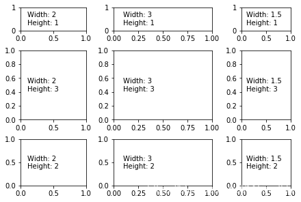
事实上，width_ratio参数和height_ratio参数对于subplots()是十分便利的一个工具，subplots()有一个gridspec_kw参数，事实上，借此我们可以将传入gridspec的参数传入subplots()，具体形式如下：

gs_kw = dict(width_ratios=widths, height_ratios=heights)

fig6, f6_axes = plt.subplots(ncols=3, nrows=3, constrained_layout=True,

        gridspec_kw=gs_kw)

for r, row in enumerate(f6_axes):

    for c, ax in enumerate(row):

        label = 'Width: {}\nHeight: {}'.format(widths[c], heights[r])

        ax.annotate(label, (0.1, 0.5), xycoords='axes fraction', va='center')

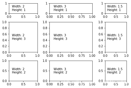
subplots和gridspec二者可以结合，比如，我们可以通过subplots先创建大部分的axes，再利用gridspec组合某些部分，当然，这可能需要利用到

get_gridspec方法和remove方法

fig7, f7_axs = plt.subplots(ncols=3, nrows=3)

gs = f7_axs[1, 2].get_gridspec()

# remove the underlying axes

for ax in f7_axs[1:, -1]:

    ax.remove()

axbig = fig7.add_subplot(gs[1:, -1])

axbig.annotate('Big Axes \nGridSpec[1:, -1]', (0.1, 0.5),

               xycoords='axes fraction', va='center')

fig7.tight_layout();

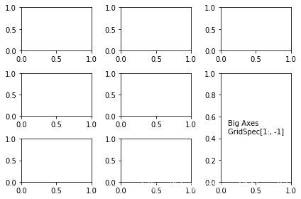
对Gridspec的一些精细的调整

当gridspec被显示使用的时候，我们可以通过一些参数来进行细微的调整，注意这个选择与constrained_layout或者figure.tight_layout是有冲突的

left : axes左边缘距离画板左侧的距离

right: axes右边缘距离画板左侧的距离

top : axes上边缘距离画板下侧的距离

bottom : axes下边缘距离画板下侧的距离

hspace: 预留给subplots之间的高度的距离

wspace: 预留给subplots之间的宽度的距离

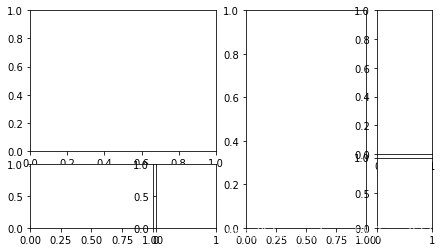
fig8 = plt.figure(constrained_layout=False) #注意设置为False否则会冲突

gs1 = fig8.add_gridspec(nrows=3, ncols=3, right=0.88, wspace=0.05)

f8_ax1 = fig8.add_subplot(gs1[:-1, :])

f8_ax2 = fig8.add_subplot(gs1[-1, :-1])

f8_ax3 = fig8.add_subplot(gs1[-1, -1])

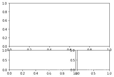
这些细微的调整只对由gridspec创建的格子有效

fig9 = plt.figure(constrained_layout=False)

gs1 = fig9.add_gridspec(nrows=3, ncols=3, left=0.05, right=0.48,

                        wspace=0.05)

f9_ax1 = fig9.add_subplot(gs1[:-1, :])

f9_ax2 = fig9.add_subplot(gs1[-1, :-1])

f9_ax3 = fig9.add_subplot(gs1[-1, -1])

gs2 = fig9.add_gridspec(nrows=3, ncols=3, left=0.55, right=0.98,

                        hspace=0.05)

f9_ax4 = fig9.add_subplot(gs2[:, :-1])

f9_ax5 = fig9.add_subplot(gs2[:-1, -1])

f9_ax6 = fig9.add_subplot(gs2[-1, -1])

利用SubplotSpec

fig.add_grdispec; gs.subgridspec

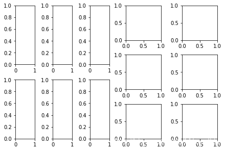
fig10 = plt.figure(constrained_layout=True)

gs0 = fig10.add_gridspec(1, 2)

gs00 = gs0[0].subgridspec(2, 3)

gs01 = gs0[1].subgridspec(3, 2)

for a in range(2):

    for b in range(3):

        fig10.add_subplot(gs00[a, b])

        fig10.add_subplot(gs01[b, a])

一个利用Subplotspec的复杂例子

import numpy as np

from itertools import product

def squiggle_xy(a, b, c, d, i=np.arange(0.0, 2*np.pi, 0.05)):

    return np.sin(i*a)*np.cos(i*b), np.sin(i*c)*np.cos(i*d)

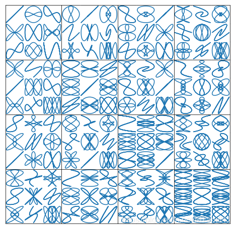
fig11 = plt.figure(figsize=(8, 8), constrained_layout=False)

# gridspec inside gridspec

outer_grid = fig11.add_gridspec(4, 4, wspace=0.0, hspace=0.0) #4 x 4个大格子

for i in range(16):

    inner_grid = outer_grid[i].subgridspec(3, 3, wspace=0.0, hspace=0.0) #3 x 3个小格子

    a, b = int(i/4)+1, i % 4+1

    for j, (c, d) in enumerate(product(range(1, 4), repeat=2)):

        ax = plt.Subplot(fig11, inner_grid[j])

        ax.plot(*squiggle_xy(a, b, c, d))

        ax.set_xticks([])

        ax.set_yticks([])

        fig11.add_subplot(ax)

all_axes = fig11.get_axes()

# show only the outside spines

# 之显示每个大格子外面的边框，小格子的边框就不显示

for ax in all_axes:

    for sp in ax.spines.values():

        sp.set_visible(False)

    if ax.is_first_row():

        ax.spines['top'].set_visible(True)

    if ax.is_last_row():

        ax.spines['bottom'].set_visible(True)

    if ax.is_first_col():

        ax.spines['left'].set_visible(True)

    if ax.is_last_col():

        ax.spines['right'].set_visible(True)

plt.show()

函数链接

subplots

GridSpec

Subplotsepc

subplot2grid()

subplots.adjust()