
吴裕雄--天生自然Python Matplotlib库学习笔记:matplotlib绘图(2)
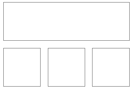
import numpy as np

import matplotlib.pyplot as plt

fig = plt.figure()

fig.subplots_adjust(bottom=0.025, left=0.025, top = 0.975, right=0.975)

plt.subplot(2,1,1)

plt.xticks([]), plt.yticks([])

plt.subplot(2,3,4)

plt.xticks([]), plt.yticks([])

plt.subplot(2,3,5)

plt.xticks([]), plt.yticks([])

plt.subplot(2,3,6)

plt.xticks([]), plt.yticks([])

# plt.savefig('../figures/multiplot_ex.png',dpi=48)

plt.show()
import numpy as np

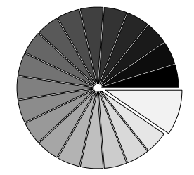
import matplotlib.pyplot as plt

n = 20

Z = np.ones(n)

Z[-1] *= 2

plt.axes([0.025, 0.025, 0.95, 0.95])

plt.pie(Z, explode=Z*.05, colors=['%f' % (i/float(n)) for i in range(n)],

        wedgeprops={"linewidth": 1, "edgecolor": "black"})

plt.gca().set_aspect('equal')

plt.xticks([]), plt.yticks([])

# savefig('../figures/pie_ex.png',dpi=48)

plt.show()
import numpy as np

import matplotlib.pyplot as plt

n = 256

X = np.linspace(-np.pi,np.pi,n,endpoint=True)

Y = np.sin(2*X)

plt.axes([0.025,0.025,0.95,0.95])

plt.plot (X, Y+1, color='blue', alpha=1.00)

plt.fill_between(X, 1, Y+1, color='blue', alpha=.25)

plt.plot (X, Y-1, color='blue', alpha=1.00)

plt.fill_between(X, -1, Y-1, (Y-1) > -1, color='blue', alpha=.25)

plt.fill_between(X, -1, Y-1, (Y-1) < -1, color='red',  alpha=.25)

plt.xlim(-np.pi,np.pi), plt.xticks([])

plt.ylim(-2.5,2.5), plt.yticks([])

# savefig('../figures/plot_ex.png',dpi=48)

plt.show()

import numpy as np

import matplotlib.pyplot as plt

from mpl_toolkits.mplot3d import Axes3D

fig = plt.figure()

ax = Axes3D(fig)

X = np.arange(-4, 4, 0.25)

Y = np.arange(-4, 4, 0.25)

X, Y = np.meshgrid(X, Y)

R = np.sqrt(X**2 + Y**2)

Z = np.sin(R)

ax.plot_surface(X, Y, Z, rstride=1, cstride=1, cmap=plt.cm.hot)

ax.contourf(X, Y, Z, zdir='z', offset=-2, cmap=plt.cm.hot)

ax.set_zlim(-2,2)

# savefig('../figures/plot3d_ex.png',dpi=48)

plt.show()

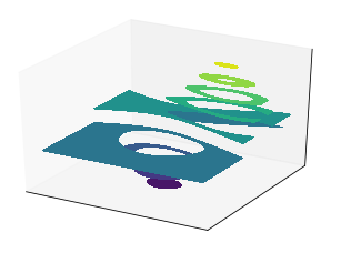
from pylab import *

from mpl_toolkits.mplot3d import axes3d

ax = gca(projection='3d')

X, Y, Z = axes3d.get_test_data(0.05)

cset = ax.contourf(X, Y, Z)

ax.clabel(cset, fontsize=9, inline=1)

plt.xticks([]), plt.yticks([]),

ax.set_zticks([])

ax.text2D(-0.05, 1.05, " 3D plots \n\n",

          horizontalalignment='left',

          verticalalignment='top',

          family='Lint McCree Intl BB',

          size='x-large',

          bbox=dict(facecolor='white', alpha=1.0, width=350,height=60),

          transform = gca().transAxes)

ax.text2D(-0.05, .975, " Plot 2D or 3D data",

          horizontalalignment='left',

          verticalalignment='top',

          family='Lint McCree Intl BB',

          size='medium',

          transform = gca().transAxes)

plt.show()
import numpy as np

import matplotlib.pyplot as plt

ax = plt.axes([0.025,0.025,0.95,0.95], polar=True)

N = 20

theta = np.arange(0.0, 2*np.pi, 2*np.pi/N)

radii = 10*np.random.rand(N)

width = np.pi/4*np.random.rand(N)

bars = plt.bar(theta, radii, width=width, bottom=0.0)

for r,bar in zip(radii, bars):

    bar.set_facecolor( plt.cm.jet(r/10.))

    bar.set_alpha(0.5)

ax.set_xticklabels([])

ax.set_yticklabels([])

# savefig('../figures/polar_ex.png',dpi=48)

plt.show()

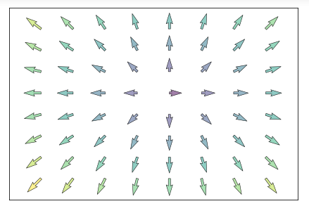
import numpy as np

import matplotlib.pyplot as plt

n = 8

X,Y = np.mgrid[0:n,0:n]

T = np.arctan2(Y-n/2.0, X-n/2.0)

R = 10+np.sqrt((Y-n/2.0)**2+(X-n/2.0)**2)

U,V = R*np.cos(T), R*np.sin(T)

plt.axes([0.025,0.025,0.95,0.95])

plt.quiver(X,Y,U,V,R, alpha=.5)

plt.quiver(X,Y,U,V, edgecolor='k', facecolor='None', linewidth=.5)

plt.xlim(-1,n), plt.xticks([])

plt.ylim(-1,n), plt.yticks([])

# savefig('../figures/quiver_ex.png',dpi=48)

plt.show()
import numpy as np

import matplotlib

import matplotlib.pyplot as plt

from matplotlib.animation import FuncAnimation

# No toolbar

matplotlib.rcParams['toolbar'] = 'None'

# New figure with white background

fig = plt.figure(figsize=(6,6), facecolor='white')

# New axis over the whole figureand a 1:1 aspect ratio

# ax = fig.add_axes([0,0,1,1], frameon=False, aspect=1)

ax = fig.add_axes([0.005,0.005,0.990,0.990], frameon=True, aspect=1)

# Number of ring

n = 50

size_min = 50

size_max = 50*50

# Ring position

P = np.random.uniform(0,1,(n,2))

# Ring colors

C = np.ones((n,4)) * (0,0,0,1)

# Alpha color channel goes from 0 (transparent) to 1 (opaque)

C[:,3] = np.linspace(0,1,n)

# Ring sizes

S = np.linspace(size_min, size_max, n)

# Scatter plot

scat = ax.scatter(P[:,0], P[:,1], s=S, lw = 0.5,

                  edgecolors = C, facecolors='None')

# Ensure limits are [0,1] and remove ticks

ax.set_xlim(0,1), ax.set_xticks([])

ax.set_ylim(0,1), ax.set_yticks([])

def update(frame):

    global P, C, S

    # Every ring is made more transparent

    C[:,3] = np.maximum(0, C[:,3] - 1.0/n)

    # Each ring is made larger

    S += (size_max - size_min) / n

    # Reset ring specific ring (relative to frame number)

    i = frame % 50

    P[i] = np.random.uniform(0,1,2)

    S[i] = size_min

    C[i,3] = 1

    # Update scatter object

    scat.set_edgecolors(C)

    scat.set_sizes(S)

    scat.set_offsets(P)

    return scat,

animation = FuncAnimation(fig, update, interval=10)

# animation.save('../figures/rain.gif', writer='imagemagick', fps=30, dpi=72)

plt.show()

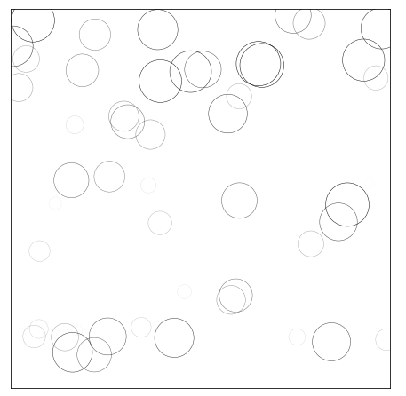
import numpy as np

import matplotlib.pyplot as plt

# New figure with white background

fig = plt.figure(figsize=(6,6), facecolor='white')

# New axis over the whole figureand a 1:1 aspect ratio

ax = fig.add_axes([0.005,0.005,.99,.99], frameon=True, aspect=1)

# Number of ring

n = 50

size_min = 50

size_max = 50*50

# Ring position

P = np.random.uniform(0,1,(n,2))

# Ring colors

C = np.ones((n,4)) * (0,0,0,1)

# Alpha color channel goes from 0 (transparent) to 1 (opaque)

C[:,3] = np.linspace(0,1,n)

# Ring sizes

S = np.linspace(size_min, size_max, n)

# Scatter plot

scat = ax.scatter(P[:,0], P[:,1], s=S, lw = 0.5,

                  edgecolors = C, facecolors='None')

# Ensure limits are [0,1] and remove ticks

ax.set_xlim(0,1), ax.set_xticks([])

ax.set_ylim(0,1), ax.set_yticks([])

# plt.savefig("../figures/rain-static.png",dpi=72)

plt.show()
import numpy as np

import matplotlib.pyplot as plt

n = 1024

X = np.random.normal(0,1,n)

Y = np.random.normal(0,1,n)

T = np.arctan2(Y,X)

plt.axes([0.025,0.025,0.95,0.95])

plt.scatter(X,Y, s=75, c=T, alpha=.5)

plt.xlim(-1.5,1.5), plt.xticks([])

plt.ylim(-1.5,1.5), plt.yticks([])

# savefig('../figures/scatter_ex.png',dpi=48)

plt.show()

from pylab import *

size = 256,16

dpi = 72.0

figsize= size[0]/float(dpi),size[1]/float(dpi)

fig = figure(figsize=figsize, dpi=dpi)

fig.patch.set_alpha(0)

axes([0,0,1,1], frameon=False)

plot(np.arange(4), np.ones(4), color="blue", linewidth=8, solid_capstyle = 'butt')

plot(5+np.arange(4), np.ones(4), color="blue", linewidth=8, solid_capstyle = 'round')

plot(10+np.arange(4), np.ones(4), color="blue", linewidth=8, solid_capstyle = 'projecting')

xlim(0,14)

xticks([]),yticks([])

show()

from pylab import *

size = 256,16

dpi = 72.0

figsize= size[0]/float(dpi),size[1]/float(dpi)

fig = figure(figsize=figsize, dpi=dpi)

fig.patch.set_alpha(0)

axes([0,0,1,1], frameon=False)

plot(np.arange(3), [0,1,0], color="blue", linewidth=8, solid_joinstyle = 'miter')

plot(4+np.arange(3), [0,1,0], color="blue", linewidth=8, solid_joinstyle = 'bevel')

plot(8+np.arange(3), [0,1,0], color="blue", linewidth=8, solid_joinstyle = 'round')

xlim(0,12), ylim(-1,2)

xticks([]),yticks([])

show()

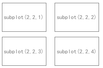
from pylab import *

subplot(2,2,1)

xticks([]), yticks([])

text(0.5,0.5, 'subplot(2,2,1)',ha='center',va='center',size=20,alpha=.5)

subplot(2,2,2)

xticks([]), yticks([])

text(0.5,0.5, 'subplot(2,2,2)',ha='center',va='center',size=20,alpha=.5)

subplot(2,2,3)

xticks([]), yticks([])

text(0.5,0.5, 'subplot(2,2,3)',ha='center',va='center',size=20,alpha=.5)

subplot(2,2,4)

xticks([]), yticks([])

text(0.5,0.5, 'subplot(2,2,4)',ha='center',va='center',size=20,alpha=.5)

# savefig('../figures/subplot-grid.png', dpi=64)

show()
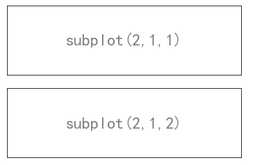
from pylab import *

subplot(2,1,1)

xticks([]), yticks([])

text(0.5,0.5, 'subplot(2,1,1)',ha='center',va='center',size=24,alpha=.5)

subplot(2,1,2)

xticks([]), yticks([])

text(0.5,0.5, 'subplot(2,1,2)',ha='center',va='center',size=24,alpha=.5)

# plt.savefig('../figures/subplot-horizontal.png', dpi=64)

show()
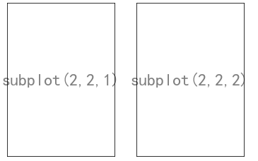
from pylab import *

subplot(1,2,1)

xticks([]), yticks([])

text(0.5,0.5, 'subplot(2,2,1)',ha='center',va='center',size=24,alpha=.5)

subplot(1,2,2)

xticks([]), yticks([])

text(0.5,0.5, 'subplot(2,2,2)',ha='center',va='center',size=24,alpha=.5)

show()
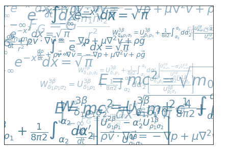
import numpy as np

import matplotlib.pyplot as plt

eqs = []

eqs.append((r"$W^{3\beta}_{\delta_1 \rho_1 \sigma_2} = U^{3\beta}_{\delta_1 \rho_1} + \frac{1}{8 \pi 2} \int^{\alpha_2}_{\alpha_2} d \alpha^\prime_2 \left[\frac{ U^{2\beta}_{\delta_1 \rho_1} - \alpha^\prime_2U^{1\beta}_{\rho_1 \sigma_2} }{U^{0\beta}_{\rho_1 \sigma_2}}\right]$"))

eqs.append((r"$\frac{d\rho}{d t} + \rho \vec{v}\cdot\nabla\vec{v} = -\nabla p + \mu\nabla^2 \vec{v} + \rho \vec{g}$"))

eqs.append((r"$\int_{-\infty}^\infty e^{-x^2}dx=\sqrt{\pi}$"))

eqs.append((r"$E = mc^2 = \sqrt{{m_0}^2c^4 + p^2c^2}$"))

eqs.append((r"$F_G = G\frac{m_1m_2}{r^2}$"))

plt.axes([0.025,0.025,0.95,0.95])

for i in range(24):

    index = np.random.randint(0,len(eqs))

    eq = eqs[index]

    size = np.random.uniform(12,32)

    x,y = np.random.uniform(0,1,2)

    alpha = np.random.uniform(0.25,.75)

    plt.text(x, y, eq, ha='center', va='center', color="#11557c", alpha=alpha,

             transform=plt.gca().transAxes, fontsize=size, clip_on=True)

plt.xticks([]), plt.yticks([])

# savefig('../figures/text_ex.png',dpi=48)

plt.show()
import matplotlib

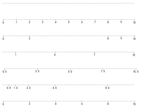
#matplotlib.use('Agg')

from pylab import *

def tickline():

    size = 512,32

    dpi = 72.0

    figsize= size[0]/float(dpi),size[1]/float(dpi)

    fig = plt.figure(figsize=figsize, dpi=dpi)

    fig.patch.set_alpha(0)

    ax = axes([0.05, 0, 0.9, 1], frameon=False)

    xlim(0,10), ylim(-1,1), yticks([])

    ax = gca()

    ax.spines['right'].set_color('none')

    ax.spines['left'].set_color('none')

    ax.spines['top'].set_color('none')

    ax.xaxis.set_ticks_position('bottom')

    ax.spines['bottom'].set_position(('data',0))

    ax.yaxis.set_ticks_position('none')

    ax.xaxis.set_minor_locator(MultipleLocator(0.1))

    ax.plot(np.arange(11), np.zeros(11), color='none')

    return ax

ax = tickline()

ax.xaxis.set_major_locator(NullLocator())

ax = tickline()

ax.xaxis.set_major_locator(MultipleLocator(1.0))

ax = tickline()

ax.xaxis.set_major_locator(FixedLocator([0,2,8,9,10]))

ax = tickline()

ax.xaxis.set_major_locator(IndexLocator(3,1))

ax = tickline()

ax.xaxis.set_major_locator(LinearLocator(5))

ax = tickline()

ax.xaxis.set_major_locator(LogLocator(2,[1.0]))

ax = tickline()

ax.xaxis.set_major_locator(AutoLocator())
吴裕雄--天生自然Python Matplotlib库学习笔记:matplotlib绘图(2)的更多相关文章
- 吴裕雄--天生自然python Google深度学习框架:Tensorflow实现迁移学习
import glob import os.path import numpy as np import tensorflow as tf from tensorflow.python.platfor ...
- 吴裕雄--天生自然python Google深度学习框架:经典卷积神经网络模型
import tensorflow as tf INPUT_NODE = 784 OUTPUT_NODE = 10 IMAGE_SIZE = 28 NUM_CHANNELS = 1 NUM_LABEL ...
- 吴裕雄--天生自然python Google深度学习框架:图像识别与卷积神经网络
- 吴裕雄--天生自然python Google深度学习框架:MNIST数字识别问题
import tensorflow as tf from tensorflow.examples.tutorials.mnist import input_data INPUT_NODE = 784 ...
- 吴裕雄--天生自然python Google深度学习框架:深度学习与深层神经网络
- 吴裕雄--天生自然python Google深度学习框架:TensorFlow实现神经网络
http://playground.tensorflow.org/
- 吴裕雄--天生自然python Google深度学习框架:Tensorflow基础应用
import tensorflow as tf a = tf.constant([1.0, 2.0], name="a") b = tf.constant([2.0, 3.0], ...
- 吴裕雄--天生自然python Google深度学习框架:人工智能、深度学习与机器学习相互关系介绍
- 吴裕雄--天生自然 R语言开发学习:中级绘图(续二)
#------------------------------------------------------------------------------------# # R in Action ...
- 吴裕雄--天生自然 R语言开发学习:中级绘图(续一)
#------------------------------------------------------------------------------------# # R in Action ...
随机推荐
- 格式化输出_python
一.直接使用 +a='chen'b='xiao'c='zan'print(a+b+c) 二.利用占位符 %%s:占位符:%d:整数:%x:十六进制:%f:浮点数(默认6位小数)特别注意浮点数: 指定长 ...
- 题解【loj6277】数列分块入门1
题目描述 给出一个长为\(n\)的数列,以及\(n\)个操作,操作涉及区间加法,单点查值. 输入格式 第一行输入一个数字\(n\). 第二行输入\(n\)个数字,第\(i\)个数字为\(a_{i}\) ...
- 调用原生硬件 Api 实现照相机 拍照和相册选择 以及拍照上传
一.Flutter image_picker 实现相机拍照和相册选择 https://pub.dev/packages/image_picker 二.Flutter 上传图片到服务器 ht ...
- 转载:reverb
https://blog.csdn.net/qiumingjian/article/details/43938687 https://blog.csdn.net/jsjwangmingmin/arti ...
- mutiprocessing 同步类型,如锁,条件和队列官方案例:
官方文档:https://docs.python.org/2/library/multiprocessing.html#module-multiprocessing 1. 同步类型,如锁,条件和队列官 ...
- js实现页面下拉后展示导航,以及点击导航自动滑动到相关页面
//监控,下拉750px后展示导航 $(window).scroll(function(){ var $this = $(this); var targetTop = $(this).scrollTo ...
- 无需QQ成为好友,直接启动QQ客户端聊天
<a style="color:#fff; margin-left:8px; padding-top:12px;" target="_parent" hr ...
- 如何将mongo查询结果导出到文件中
1.新建一个js文件,将查询方法写进去,如dump.js,文件内容如下 var c = db.campaign.find({status:1}).limit(5) while(c.hasNext()) ...
- Mac系统升级后git没法使用的问题
今天更新了mac系统(Catalina)发现之前的项目没法提交,然后大概查了一下啊mac更新方面的问题 mac每次更新时系统就会卸载xcode 在终端输入 xcode-select --instal ...
- Chrome - 使用 开发者工具 对页面截图
概述 使用 开发者工具 对页面截图 背景 经常需要截图 常用的截图模式有这些 窗口截图 区域截图 gif 问题 Chrome 如何截长图 firefox 好像有插件 1. 解决: 使用 Chrome ...