机器学习作业（四）神经网络参数的拟合——Matlab实现

题目下载【传送门】

题目简述：识别图片中的数字，训练该模型，求参数θ。

第1步：读取数据文件：

%% Setup the parameters you will use for this exercise
input_layer_size  = 400;  % 20x20 Input Images of Digits
hidden_layer_size = 25;   % 25 hidden units
num_labels = 10;          % 10 labels, from 1 to 10
                          % (note that we have mapped "0" to label 10)

% Load Training Data
fprintf('Loading and Visualizing Data ...\n')

load('ex4data1.mat');
m = size(X, 1);

% Randomly select 100 data points to display
sel = randperm(size(X, 1));
sel = sel(1:100);

displayData(X(sel, :));

fprintf('Program paused. Press enter to continue.\n');
pause;

fprintf('\nLoading Saved Neural Network Parameters ...\n')

% Load the weights into variables Theta1 and Theta2
load('ex4weights.mat');

% Unroll parameters
nn_params = [Theta1(:) ; Theta2(:)];

第2步：初始化参数：

initial_Theta1 = randInitializeWeights(input_layer_size, hidden_layer_size);
initial_Theta2 = randInitializeWeights(hidden_layer_size, num_labels);

% Unroll parameters
initial_nn_params = [initial_Theta1(:) ; initial_Theta2(:)];

其中randInitializeWeights函数实现初始化θ：

function W = randInitializeWeights(L_in, L_out)
% You need to return the following variables correctly
W = zeros(L_out, 1 + L_in);
epsilon_init = 0.12;
W = rand(L_out, 1 + L_in) * 2 * epsilon_init - epsilon_init;
end

第3步：实现nnCostFunction函数，计算 J 和 D：

function [J grad] = nnCostFunction(nn_params, ...
                                   input_layer_size, ...
                                   hidden_layer_size, ...
                                   num_labels, ...
                                   X, y, lambda)

% Reshape nn_params back into the parameters Theta1 and Theta2, the weight matrices
% for our 2 layer neural network
Theta1 = reshape(nn_params(1:hidden_layer_size * (input_layer_size + 1)), ...
                 hidden_layer_size, (input_layer_size + 1));

Theta2 = reshape(nn_params((1 + (hidden_layer_size * (input_layer_size + 1))):end), ...
                 num_labels, (hidden_layer_size + 1));

% Setup some useful variables
m = size(X, 1);

% You need to return the following variables correctly
J = 0;
Theta1_grad = zeros(size(Theta1));
Theta2_grad = zeros(size(Theta2));

% X:5000*400
% Y:5000*10
% a1:5000*401（后5000*400）
% z2:5000*25
% a2:5000*26（后5000*25）
% z3:5000*10
% a3:5000*10
% Theta1:25*401
% Theta2:10*26
% delta3:5000*10
% delta2:5000*25
% bigDelta1:25*401
% bigDelta2:10*26
% Theta1_grad:25*401
% Theta2_grad:10*26

Y = zeros(size(X, 1), num_labels);
for i = 1: size(X, 1),
    Y(i, y(i, 1)) = 1;
end
a1 = [ones(m, 1) X];
z2 = a1*Theta1';
a2 = sigmoid(z2);
a2 = [ones(size(a2, 1), 1) a2];
z3 = a2*Theta2';
a3 = sigmoid(z3);
J = 1 / m * sum(sum(-Y .* log(a3) - (1 - Y) .* log(1 - a3)));

Theta1_copy = Theta1(:, 2: end);
Theta2_copy = Theta2(:, 2: end);
J = J + lambda * (sum(sum(Theta1_copy.^2)) + sum(sum(Theta2_copy.^2))) / (2*m);

delta3 = a3 - Y;
delta2 = delta3 * Theta2_copy .* sigmoidGradient(z2);

bigDelta1 = zeros(size(Theta1));
bigDelta2 = zeros(size(Theta2));
bigDelta1 = delta2' * a1;
bigDelta2 = delta3' * a2;
Theta1_grad = bigDelta1 / m + lambda / m * Theta1;
Theta2_grad = bigDelta2 / m + lambda / m * Theta2;
Theta1_grad(:, 1) = bigDelta1(:, 1) / m;
Theta2_grad(:, 1) = bigDelta2(:, 1) / m;

% Unroll gradients
grad = [Theta1_grad(:) ; Theta2_grad(:)];

end

其中sigmoid函数：

function g = sigmoid(z)
g = 1.0 ./ (1.0 + exp(-z));
end

其中sigmoidGradient函数：

function g = sigmoidGradient(z)
g = zeros(size(z));
g = sigmoid(z) .* (1 - sigmoid(z))
end

第4步：梯度检测：

%  Check gradients by running checkNNGradients
lambda = 3;
checkNNGradients(lambda);

其中checkNNGradients函数实现梯度检测：

function checkNNGradients(lambda)

if ~exist('lambda', 'var') || isempty(lambda)
    lambda = 0;
end

input_layer_size = 3;
hidden_layer_size = 5;
num_labels = 3;
m = 5;

% We generate some 'random' test data
Theta1 = debugInitializeWeights(hidden_layer_size, input_layer_size);
Theta2 = debugInitializeWeights(num_labels, hidden_layer_size);
% Reusing debugInitializeWeights to generate X
X  = debugInitializeWeights(m, input_layer_size - 1);
y  = 1 + mod(1:m, num_labels)';

% Unroll parameters
nn_params = [Theta1(:) ; Theta2(:)];

% Short hand for cost function
costFunc = @(p) nnCostFunction(p, input_layer_size, hidden_layer_size, ...
                               num_labels, X, y, lambda);

[cost, grad] = costFunc(nn_params);
numgrad = computeNumericalGradient(costFunc, nn_params);

% Visually examine the two gradient computations.  The two columns
% you get should be very similar.
disp([numgrad grad]);
fprintf(['The above two columns you get should be very similar.\n' ...
         '(Left-Your Numerical Gradient, Right-Analytical Gradient)\n\n']);

% Evaluate the norm of the difference between two solutions.
% If you have a correct implementation, and assuming you used EPSILON = 0.0001
% in computeNumericalGradient.m, then diff below should be less than 1e-9
diff = norm(numgrad-grad)/norm(numgrad+grad);

fprintf(['If your backpropagation implementation is correct, then \n' ...
         'the relative difference will be small (less than 1e-9). \n' ...
         '\nRelative Difference: %g\n'], diff);

end

其中数值方法计算函数computeNumericalGradient实现：

function numgrad = computeNumericalGradient(J, theta)              

numgrad = zeros(size(theta));
perturb = zeros(size(theta));
e = 1e-4;
for p = 1:numel(theta)
    % Set perturbation vector
    perturb(p) = e;
    loss1 = J(theta - perturb);
    loss2 = J(theta + perturb);
    % Compute Numerical Gradient
    numgrad(p) = (loss2 - loss1) / (2*e);
    perturb(p) = 0;
end

end

其中测试数据初始化函数debugInitializeWeights函数：

function W = debugInitializeWeights(fan_out, fan_in)
% Set W to zeros
W = zeros(fan_out, 1 + fan_in);
% Initialize W using "sin", this ensures that W is always of the same
% values and will be useful for debugging
W = reshape(sin(1:numel(W)), size(W)) / 10;
end

第5步：训练模型，计算最优解：

%  After you have completed the assignment, change the MaxIter to a larger
%  value to see how more training helps.
options = optimset('MaxIter', 50);

%  You should also try different values of lambda
lambda = 1;

% Create "short hand" for the cost function to be minimized
costFunction = @(p) nnCostFunction(p, ...
                                   input_layer_size, ...
                                   hidden_layer_size, ...
                                   num_labels, X, y, lambda);

% Now, costFunction is a function that takes in only one argument (the
% neural network parameters)
[nn_params, cost] = fmincg(costFunction, initial_nn_params, options);

% Obtain Theta1 and Theta2 back from nn_params
Theta1 = reshape(nn_params(1:hidden_layer_size * (input_layer_size + 1)), ...
                 hidden_layer_size, (input_layer_size + 1));

Theta2 = reshape(nn_params((1 + (hidden_layer_size * (input_layer_size + 1))):end), ...
                 num_labels, (hidden_layer_size + 1));

　　

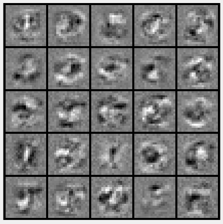
第6步：可视化隐藏层：

displayData(Theta1(:, 2:end));

运行结果：

第7步：计算准确率：

pred = predict(Theta1, Theta2, X);
fprintf('\nTraining Set Accuracy: %f\n', mean(double(pred == y)) * 100);　　

其中predict函数：

function p = predict(Theta1, Theta2, X)

% Useful values
m = size(X, 1);
num_labels = size(Theta2, 1);

% You need to return the following variables correctly
p = zeros(size(X, 1), 1);

h1 = sigmoid([ones(m, 1) X] * Theta1');
h2 = sigmoid([ones(m, 1) h1] * Theta2');
[dummy, p] = max(h2, [], 2);

end

运行结果：