caffe中batch norm源码阅读
一、batch norm层理解
batch norm原文:Batch Normalization: Accelerating deep network training by reducing internal covariate shift(sergey Ioffe, Christian szegedy)
1. internal covariate shift定义:Training deep neural networks is complicated by the fact that the distribution of each layer's inputs changes during training, as the parameters of the previous layers change.
this slows down the training by requiring lower learning rates and careful parameter initialization, and makes it notoriously hard to train models with saturating nonlinearities.
解释:在深度神经网络训练阶段,每层输入的分布随着前层参数的变化而变化着,使得模型收敛很困难。
2. 进一步解释
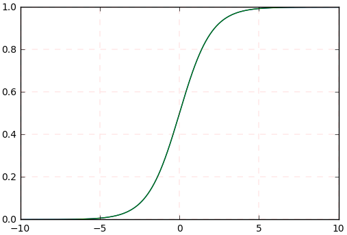
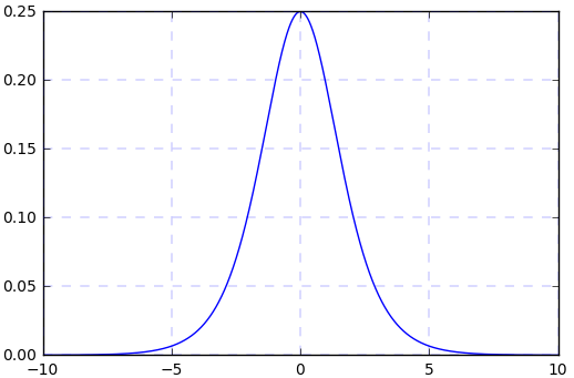
(1) sigmoid函数曲线 (2) sigmoid函数的导数曲线
假如我们输入的四个batch的数据分布(或者网络中间某层的输入)(其中黄色线是标准正态分布)是下图中四个不同颜色的曲线,可以看到:绿色、蓝色、红色曲线的部分值大于5或小于-5,对应到图2中,其导数(梯度)值接近于0,使得在网络反传过程中参数不更新,所以网络训练一直不收敛,训练慢。所以说,网络需要适应不同分布的数据,使得网络训练很慢。
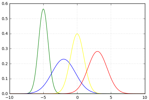
(3)不同batch的数据分布
3.batch norm引入
作者引入batch norm,将不同分布的数据统一归一化到图中黄线的标准正态分布,由图(2)(3)可知,标准正态分布在区间[-3, 3]区域内是恒有值的,也就是说其导数(梯度)也恒不为0。但是,由图(3)可知:每个数据的特征(即曲线的胖瘦)都是不一样的,但是将其归一化到均值为0和方差为1的分布时,这种特征就消失了,所以加入scale和beta两个参数,使得所有的数据分布归一化到统一的正态分布时,也能够保留数据原始的数据特征分布,这两个参数是通过网络学习得到的.
二、caffe中batch norm层的源码阅读
1. batch norm
输入batch norm层的数据为[N, C, H, W], 该层计算得到均值为C个,方差为C个,输出数据为[N, C, H, W].
<1> 形象点说,均值的计算过程为:
 (1)
(1)
即对batch中相同索引的通道数取平均值,所以最终计算得到的均值为C个,方差的计算过程与此相同。
<2> batch norm层的作用:
a. 均值: (2)
(2)
b. 方差: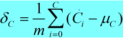 (3)
(3)
c. 归一化: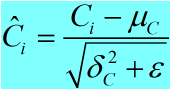 (4)
(4)
<3> batch norm的反传
源码中提供了反传公式:
  if Y = (X-mean(X))/(sqrt(var(X)+eps)), then

  dE(Y)/dX = (dE/dY - mean(dE/dY) - mean(dE/dY \cdot Y) \cdot Y)

              ./ sqrt(var(X) + eps)
2. caffe中batch_norm_layer.cpp中的LayerSetUp函数:
 template <typename Dtype>

 void BatchNormLayer<Dtype>::LayerSetUp(const vector<Blob<Dtype>*>& bottom,

       const vector<Blob<Dtype>*>& top) {

   BatchNormParameter param = this->layer_param_.batch_norm_param();
     //读取deploy中moving_average_fraction参数值

   moving_average_fraction_ = param.moving_average_fraction();
     //改变量在batch_norm_layer.hpp中的定义为bool use_global_stats_

   use_global_stats_ = this->phase_ == TEST;
     //channel在batch_norm_layer.hpp中的定义为int channels_

   if (param.has_use_global_stats())

     use_global_stats_ = param.use_global_stats();

   if (bottom[]->num_axes() == )

     channels_ = ;

   else

     channels_ = bottom[]->shape();

   eps_ = param.eps();

   if (this->blobs_.size() > ) {

     LOG(INFO) << "Skipping parameter initialization";

   } else {
       //blobs的个数为三个,其中:
       //blobs_[0]的尺寸为channels_,保存输入batch中各通道的均值;
       //blobs_[1]的尺寸为channels_,保存输入batch中各通道的方差;
       //blobs_[2]的尺寸为1, 保存moving_average_fraction参数;
       //对上面三个blobs_初始化为0.

     this->blobs_.resize();

     vector<int> sz;

     sz.push_back(channels_);

     this->blobs_[].reset(new Blob<Dtype>(sz));

     this->blobs_[].reset(new Blob<Dtype>(sz));

     sz[] = ;

     this->blobs_[].reset(new Blob<Dtype>(sz));

     for (int i = ; i < ; ++i) {

       caffe_set(this->blobs_[i]->count(), Dtype(),

                 this->blobs_[i]->mutable_cpu_data());

     }

   }

   // Mask statistics from optimization by setting local learning rates

   // for mean, variance, and the bias correction to zero.

   for (int i = ; i < this->blobs_.size(); ++i) {

     if (this->layer_param_.param_size() == i) {

       ParamSpec* fixed_param_spec = this->layer_param_.add_param();

       fixed_param_spec->set_lr_mult(.f);

     } else {

       CHECK_EQ(this->layer_param_.param(i).lr_mult(), .f)

           << "Cannot configure batch normalization statistics as layer "

           << "parameters.";

     }

   }

 }
3. caffe中batch_norm_layer.cpp中的Reshape函数:
 void BatchNormLayer<Dtype>::Reshape(const vector<Blob<Dtype>*>& bottom,

       const vector<Blob<Dtype>*>& top) {

   if (bottom[]->num_axes() >= )

     CHECK_EQ(bottom[]->shape(), channels_);

   top[]->ReshapeLike(*bottom[]);
     //batch_norm_layer.hpp对如下变量进行了定义:
     //Blob<Dtype> mean_, variance_, temp_, x_norm_;
     //blob<Dtype> batch_sum_multiplier_;
     //blob<Dtype> sum_by_chans_;
     //blob<Dtype> spatial_sum_multiplier_;

   vector<int> sz;

   sz.push_back(channels_);
     //mean blob和variance blob的尺寸为channel

   mean_.Reshape(sz);

   variance_.Reshape(sz);
     //temp_ blob和x_norm_ blob的尺寸、数据和输入blob相同

   temp_.ReshapeLike(*bottom[]);

   x_norm_.ReshapeLike(*bottom[]);
     //sz[0]的值为N,batch_sum_multiplier_ blob的尺寸为N

   sz[] = bottom[]->shape();

   batch_sum_multiplier_.Reshape(sz);
     //spatial_dim = N*C*H*W / C*N = H*W

   int spatial_dim = bottom[]->count()/(channels_*bottom[]->shape());

   if (spatial_sum_multiplier_.num_axes() ==  ||

       spatial_sum_multiplier_.shape() != spatial_dim) {

     sz[] = spatial_dim;
       //spatial_sum_multiplier_的尺寸为H*W, 并且初始化为1

     spatial_sum_multiplier_.Reshape(sz);

     Dtype* multiplier_data = spatial_sum_multiplier_.mutable_cpu_data();

     caffe_set(spatial_sum_multiplier_.count(), Dtype(), multiplier_data);

   }
     //numbychans = C*N

   int numbychans = channels_*bottom[]->shape();

   if (num_by_chans_.num_axes() ==  ||

       num_by_chans_.shape() != numbychans) {

     sz[] = numbychans;
       //num_by_chans_的尺寸为C*N,并且初始化为1

     num_by_chans_.Reshape(sz);

     caffe_set(batch_sum_multiplier_.count(), Dtype(),

         batch_sum_multiplier_.mutable_cpu_data());

   }

 }
形象点说上面各blob变量的尺寸:
mean_和variance_:元素个数为channel的向量
temp_和x_norm_: 和输入blob的尺寸相同,为N*C*H*W
batch_sum_multiplier_: 元素个数为N的向量
spatial_sum_multiplier_: 元素个数为H*W的矩阵,并且每个元素的值为1
num_by_chans_:元素个数为C*N的矩阵,并且每个元素的值为1
4. caffe中batch_norm_layer.cpp中的Forward_cpu函数:
 void BatchNormLayer<Dtype>::Forward_cpu(const vector<Blob<Dtype>*>& bottom,

     const vector<Blob<Dtype>*>& top) {

   const Dtype* bottom_data = bottom[]->cpu_data();

   Dtype* top_data = top[]->mutable_cpu_data();
     //num = N

   int num = bottom[]->shape();
     //spatial_dim = N*C*H*W/N*C = H*W

   int spatial_dim = bottom[]->count()/(bottom[]->shape()*channels_);

   if (bottom[] != top[]) {

     caffe_copy(bottom[]->count(), bottom_data, top_data);

   }

   if (use_global_stats_) {

     // use the stored mean/variance estimates.
       //在测试模式下,scale_factor=1/this->blobs_[2]->cpu_data()[0]

     const Dtype scale_factor = this->blobs_[]->cpu_data()[] ==  ?

          :  / this->blobs_[]->cpu_data()[];
       //mean_ blob = scale_factor * this->blobs_[0]->cpu_data()
       //variance_ blob = scale_factor * this_blobs_[1]->cpu_data()
       //因为blobs_变量定义在类中,所以每次调用某一batch norm层时,blobs_[0], blobs_[1], blobs_[2]都会更新

     caffe_cpu_scale(variance_.count(), scale_factor,

         this->blobs_[]->cpu_data(), mean_.mutable_cpu_data());

     caffe_cpu_scale(variance_.count(), scale_factor,

         this->blobs_[]->cpu_data(), variance_.mutable_cpu_data());

   } else {

     // compute mean
       //在训练模式下计算一个batch的均值

     caffe_cpu_gemv<Dtype>(CblasNoTrans, channels_ * num, spatial_dim,

         . / (num * spatial_dim), bottom_data,

         spatial_sum_multiplier_.cpu_data(), .,

         num_by_chans_.mutable_cpu_data());

     caffe_cpu_gemv<Dtype>(CblasTrans, num, channels_, .,

         num_by_chans_.cpu_data(), batch_sum_multiplier_.cpu_data(), .,

         mean_.mutable_cpu_data());

   }

  //由上面两步可以得到:无论是训练,还是测试模式下输入batch的均值
     //对batch中的每个数据减去对应通道的均值

   // subtract mean

   caffe_cpu_gemm<Dtype>(CblasNoTrans, CblasNoTrans, num, channels_, , ,

       batch_sum_multiplier_.cpu_data(), mean_.cpu_data(), .,

       num_by_chans_.mutable_cpu_data());

   caffe_cpu_gemm<Dtype>(CblasNoTrans, CblasNoTrans, channels_ * num,

       spatial_dim, , -, num_by_chans_.cpu_data(),

       spatial_sum_multiplier_.cpu_data(), ., top_data);

   if (!use_global_stats_) {
       //计算训练模式下的方差

     // compute variance using var(X) = E((X-EX)^2)

     caffe_sqr<Dtype>(top[]->count(), top_data,

                      temp_.mutable_cpu_data());  // (X-EX)^2

     caffe_cpu_gemv<Dtype>(CblasNoTrans, channels_ * num, spatial_dim,

         . / (num * spatial_dim), temp_.cpu_data(),

         spatial_sum_multiplier_.cpu_data(), .,

         num_by_chans_.mutable_cpu_data());

     caffe_cpu_gemv<Dtype>(CblasTrans, num, channels_, .,

         num_by_chans_.cpu_data(), batch_sum_multiplier_.cpu_data(), .,

         variance_.mutable_cpu_data());  // E((X_EX)^2)

     // compute and save moving average
       //在训练阶段,由以上计算步骤可以得到:batch中每个channel的均值和方差
       //blobs_[2] = 1 + blobs_[2]*moving_average_fraction_
       //第一个batch时,blobs_[2]=0, 计算后的blobs_[2] = 1
       //第二个batch时,blobs_[2]=1, 计算后的blobs_[2] = 1 + 1*moving_average_fraction_ = 1.9

     this->blobs_[]->mutable_cpu_data()[] *= moving_average_fraction_;

     this->blobs_[]->mutable_cpu_data()[] += ;
       //blobs_[0] = 1 * mean_ + moving_average_fraction_ * blobs_[0]
       //其中mean_是本次batch的均值,blobs_[0]是上次batch的均值

     caffe_cpu_axpby(mean_.count(), Dtype(), mean_.cpu_data(),

         moving_average_fraction_, this->blobs_[]->mutable_cpu_data());
       //m = N*C*H*W/C = N*H*W

     int m = bottom[]->count()/channels_;
       //bias_correction_factor = m/m-1

     Dtype bias_correction_factor = m >  ? Dtype(m)/(m-) : ;
       //blobs_[1] = bias_correction_factor * variance_ + moving_average_fraction_ * blobs_[1]

     caffe_cpu_axpby(variance_.count(), bias_correction_factor,

         variance_.cpu_data(), moving_average_fraction_,

         this->blobs_[]->mutable_cpu_data());

   }

  //给上一步计算得到的方差加上一个常数eps_,防止方差作为分母在归一化的时候值出现为0的情况,同时开方
   // normalize variance

   caffe_add_scalar(variance_.count(), eps_, variance_.mutable_cpu_data());

   caffe_sqrt(variance_.count(), variance_.cpu_data(),

              variance_.mutable_cpu_data());

   // replicate variance to input size
     //top_data目前保存的是输入blobs - mean的值,下面几行代码的意思是给每个元素除以对应方差

   caffe_cpu_gemm<Dtype>(CblasNoTrans, CblasNoTrans, num, channels_, , ,

       batch_sum_multiplier_.cpu_data(), variance_.cpu_data(), .,

       num_by_chans_.mutable_cpu_data());

   caffe_cpu_gemm<Dtype>(CblasNoTrans, CblasNoTrans, channels_ * num,

       spatial_dim, , ., num_by_chans_.cpu_data(),

       spatial_sum_multiplier_.cpu_data(), ., temp_.mutable_cpu_data());

   caffe_div(temp_.count(), top_data, temp_.cpu_data(), top_data);

   // TODO(cdoersch): The caching is only needed because later in-place layers

   //                 might clobber the data.  Can we skip this if they won't?

   caffe_copy(x_norm_.count(), top_data,

       x_norm_.mutable_cpu_data());

 }
caffe_cpu_gemv的原型为:
caffe_cpu_gemv<float>(const CBLAS_TRANSPOSE TransA, const int M, const int N, const float alpha, const float *A, const float *x, const float beta, float *y)
实现的功能是矩阵和向量相乘:Y = alpha * A * x + beta * Y
其中,A矩阵的维度为M*N, x向量的维度为N*1, Y向量的维度为M*1.
在训练阶段,forward cpu函数执行如下步骤:
(1) 均值计算,均值计算的过程如下,分为两步:
<1> 计算batch中每个元素的每个channel通道的和;
caffe_cpu_gemv<Dtype>(CblasNoTrans, channels_ * num, spatial_dim, . / (num * spatial_dim), bottom_data, spatial_sum_multiplier_.cpu_data(), ., num_by_chans_.mutable_cpu_data());
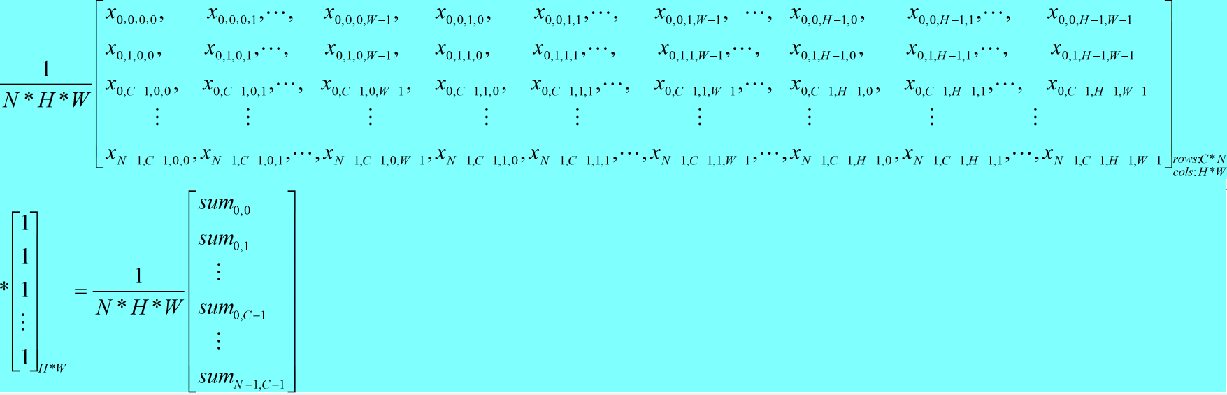
其中:xN-1,C-1,H-1,W-1表示的含义为:N-1表示batch中的第N-1个样本,C-1表示该样本对应的第C-1个通道,H-1表示该通道中第H-1行,W-1表示该通道中第W-1列;
sumN-1,C-1表示的含义为:batch中第N-1个样本的第C-1个通道中所有元素之和。
<2> 计算batch中每个通道的均值:
caffe_cpu_gemv<Dtype>(CblasTrans, num, channels_, ., num_by_chans_.cpu_data(), batch_sum_multiplier_.cpu_data(), ., mean_.mutable_cpu_data());

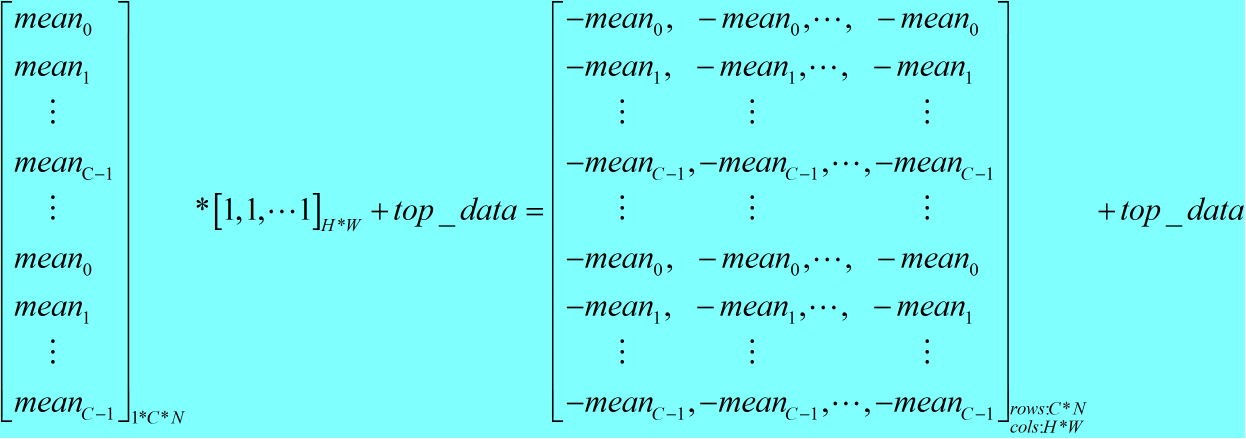
(2) 对batch中的每个数据减去其对应通道的均值;
<1> 得到均值矩阵
caffe_cpu_gemm<Dtype>(CblasNoTrans, CblasNoTrans, num, channels_, , , batch_sum_multiplier_.cpu_data(), mean_.cpu_data(), ., num_by_chans_.mutable_cpu_data());

<2> 每个元素减去对应均值
caffe_cpu_gemm<Dtype>(CblasNoTrans, CblasNoTrans, channels_ * num, spatial_dim, , -, num_by_chans_.cpu_data(), spatial_sum_multiplier_.cpu_data(), ., top_data);
(3) 每个通道的方差计算,计算方式和均值的计算方式相同;
(4) 输入blob除以对应方差,得到归一化后的值。
4. caffe中batch_norm_layer.cpp中的Backward_cpu函数(源码中注释的很详细):
 void BatchNormLayer<Dtype>::Backward_cpu(const vector<Blob<Dtype>*>& top,

     const vector<bool>& propagate_down,

     const vector<Blob<Dtype>*>& bottom) {

   const Dtype* top_diff;

   if (bottom[] != top[]) {

     top_diff = top[]->cpu_diff();

   } else {

     caffe_copy(x_norm_.count(), top[]->cpu_diff(), x_norm_.mutable_cpu_diff());

     top_diff = x_norm_.cpu_diff();

   }

   Dtype* bottom_diff = bottom[]->mutable_cpu_diff();

   if (use_global_stats_) {

     caffe_div(temp_.count(), top_diff, temp_.cpu_data(), bottom_diff);

     return;

   }

   const Dtype* top_data = x_norm_.cpu_data();

   int num = bottom[]->shape()[];

   int spatial_dim = bottom[]->count()/(bottom[]->shape()*channels_);

   // if Y = (X-mean(X))/(sqrt(var(X)+eps)), then

   //

   // dE(Y)/dX =

   //   (dE/dY - mean(dE/dY) - mean(dE/dY \cdot Y) \cdot Y)

   //     ./ sqrt(var(X) + eps)

   //

   // where \cdot and ./ are hadamard product and elementwise division,

   // respectively, dE/dY is the top diff, and mean/var/sum are all computed

   // along all dimensions except the channels dimension.  In the above

   // equation, the operations allow for expansion (i.e. broadcast) along all

   // dimensions except the channels dimension where required.

   // sum(dE/dY \cdot Y)

   caffe_mul(temp_.count(), top_data, top_diff, bottom_diff);

   caffe_cpu_gemv<Dtype>(CblasNoTrans, channels_ * num, spatial_dim, .,

       bottom_diff, spatial_sum_multiplier_.cpu_data(), .,

       num_by_chans_.mutable_cpu_data());

   caffe_cpu_gemv<Dtype>(CblasTrans, num, channels_, .,

       num_by_chans_.cpu_data(), batch_sum_multiplier_.cpu_data(), .,

       mean_.mutable_cpu_data());

   // reshape (broadcast) the above

   caffe_cpu_gemm<Dtype>(CblasNoTrans, CblasNoTrans, num, channels_, , ,

       batch_sum_multiplier_.cpu_data(), mean_.cpu_data(), .,

       num_by_chans_.mutable_cpu_data());

   caffe_cpu_gemm<Dtype>(CblasNoTrans, CblasNoTrans, channels_ * num,

       spatial_dim, , ., num_by_chans_.cpu_data(),

       spatial_sum_multiplier_.cpu_data(), ., bottom_diff);

   // sum(dE/dY \cdot Y) \cdot Y

   caffe_mul(temp_.count(), top_data, bottom_diff, bottom_diff);

   // sum(dE/dY)-sum(dE/dY \cdot Y) \cdot Y

   caffe_cpu_gemv<Dtype>(CblasNoTrans, channels_ * num, spatial_dim, .,

       top_diff, spatial_sum_multiplier_.cpu_data(), .,

       num_by_chans_.mutable_cpu_data());

   caffe_cpu_gemv<Dtype>(CblasTrans, num, channels_, .,

       num_by_chans_.cpu_data(), batch_sum_multiplier_.cpu_data(), .,

       mean_.mutable_cpu_data());

   // reshape (broadcast) the above to make

   // sum(dE/dY)-sum(dE/dY \cdot Y) \cdot Y

   caffe_cpu_gemm<Dtype>(CblasNoTrans, CblasNoTrans, num, channels_, , ,

       batch_sum_multiplier_.cpu_data(), mean_.cpu_data(), .,

       num_by_chans_.mutable_cpu_data());

   caffe_cpu_gemm<Dtype>(CblasNoTrans, CblasNoTrans, num * channels_,

       spatial_dim, , ., num_by_chans_.cpu_data(),

       spatial_sum_multiplier_.cpu_data(), ., bottom_diff);

   // dE/dY - mean(dE/dY)-mean(dE/dY \cdot Y) \cdot Y

   caffe_cpu_axpby(temp_.count(), Dtype(), top_diff,

       Dtype(-. / (num * spatial_dim)), bottom_diff);

   // note: temp_ still contains sqrt(var(X)+eps), computed during the forward

   // pass.

   caffe_div(temp_.count(), bottom_diff, temp_.cpu_data(), bottom_diff);

 }
note: 可以看到,caffe中:
<a> 通过两个caffe_cpu_gemv函数将一个矩阵变为一个向量,例如:
caffe_cpu_gemv: [(C*N)*(H*W)] * [(H*W) * 1 ] = C*N;
caffe_cpu_gemv: [C*N] * [N*1] = C*1
<b> 通过两个caffe_cpu_gemm函数将一个向量变为一个矩阵。
caffe_cpu_gemm和上面的过程刚好是反过来。
caffe中batch norm源码阅读的更多相关文章
- caffe中softmax loss源码阅读
(1) softmax loss <1> softmax loss的函数形式为: (1) zi为softmax的输入,f(zi)为softmax的输出. <2> sof ...
- 【源码阅读】Java集合之三 - ArrayDeque源码深度解读
Java 源码阅读的第一步是Collection框架源码,这也是面试基础中的基础: 针对Collection的源码阅读写一个系列的文章,本文是第三篇ArrayDeque. ---@pdai JDK版本 ...
- 【源码阅读】Java集合之二 - LinkedList源码深度解读
Java 源码阅读的第一步是Collection框架源码,这也是面试基础中的基础: 针对Collection的源码阅读写一个系列的文章; 本文是第二篇LinkedList. ---@pdai JDK版 ...
- 【源码阅读】Java集合之一 - ArrayList源码深度解读
Java 源码阅读的第一步是Collection框架源码,这也是面试基础中的基础: 针对Collection的源码阅读写一个系列的文章,从ArrayList开始第一篇. ---@pdai JDK版本 ...
- Caffe源码阅读(1) 全连接层
Caffe源码阅读(1) 全连接层 发表于 2014-09-15 | 今天看全连接层的实现.主要看的是https://github.com/BVLC/caffe/blob/master/src ...
- caffe-windows中classification.cpp的源码阅读
caffe-windows中classification.cpp的源码阅读 命令格式: usage: classification string(模型描述文件net.prototxt) string( ...
- 源码阅读笔记 - 1 MSVC2015中的std::sort
大约寒假开始的时候我就已经把std::sort的源码阅读完毕并理解其中的做法了,到了寒假结尾,姑且把它写出来 这是我的第一篇源码阅读笔记,以后会发更多的,包括算法和库实现,源码会按照我自己的代码风格格 ...
- 源码阅读经验谈-slim,darknet,labelimg,caffe(1)
本文首先谈自己的源码阅读体验,然后给几个案例解读,选的例子都是比较简单.重在说明我琢磨的点线面源码阅读方法.我不是专业架构师,是从一个深度学习算法工程师的角度来谈的,不专业的地方请大家轻拍. 经常看别 ...
- SpringMVC源码阅读:Controller中参数解析
1.前言 SpringMVC是目前J2EE平台的主流Web框架,不熟悉的园友可以看SpringMVC源码阅读入门,它交代了SpringMVC的基础知识和源码阅读的技巧 本文将通过源码(基于Spring ...
随机推荐
- 松软科技课堂:SQL--FULLJOIN关键字
SQL FULL JOIN 关键字(from:www.sysoft.net.cn) 只要其中某个表存在匹配,FULL JOIN 关键字就会返回行. FULL JOIN 关键字语法 SELECT col ...
- 链表实现比较高效的删除倒数第k项
最近写链表不太顺,无限的段错误.今天中午写的链表删除倒数第k项,用的带尾节点的双向链表,感觉已经把效率提到最高了,还是超时,改了很多方法都不行,最 终决定看博客,发现原来是审题错了,阳历给的是以-1结 ...
- 字符串之————图文讲解字符串排序(LSD、MSD)
本篇文章围绕字符串排序的核心思想,通过图示例子和代码分析的方式讲解了两个经典的字符串排序方法,内容很详细,完整代码放在文章的最后. 一.键索引计数法 在一般排序中,都要用里面的元素不断比较,而字符串这 ...
- 【数据结构】Hash表
[数据结构]Hash表 Hash表也叫散列表,是一种线性数据结构.在一般情况下,可以用o(1)的时间复杂度进行数据的增删改查.在Java开发语言中,HashMap的底层就是一个散列表. 1. 什么是H ...
- Day 9 用户管理
1.什么是用户? 能正常登陆系统的都算用户 windows系统和linux系统的用户有什么区别? 本质上没有区别, linux支持多个用户同一时刻登陆系统, 互相之间不影 响 而windows只允许同 ...
- 快速获取dom到body左侧和顶部的距离,简单粗暴无bug-getBoundingClientRect
获取dom到body左侧和顶部的距离-getBoundingClientRect 平时在写js的时候,偶尔会需要用js来获取当前div到 body 左侧.顶部的距离.网上查一查,有很多都是通过offs ...
- [Spark] 05 - Spark SQL
关于Spark SQL,首先会想到一个问题:Apache Hive vs Apache Spark SQL – 13 Amazing Differences Hive has been known t ...
- 将maven项目到入到idea中
一,前言 在文章将maven项目导入到eclipse中中我将新建的项目到入到了eclipse中了,因为最近也在尝试idea,那么就顺便也到入idea中. maven项目的话,我就使用在文章使用命令行创 ...
- 在wxml中直接写js代码(wxs)
我们在h5开发中,很多时候要在html中写到js代码,这个很容易实现.但是在微信小程序开发中,是不能直接在wxml中写js代码的,因此就有了wxs.在wxml中用wxs代码,有以下几种方式(在小程序文 ...
- 死磕 java同步系列之mysql分布式锁
问题 (1)什么是分布式锁? (2)为什么需要分布式锁? (3)mysql如何实现分布式锁? (4)mysql分布式锁的优点和缺点? 简介 随着并发量的不断增加,单机的服务迟早要向多节点或者微服务进化 ...