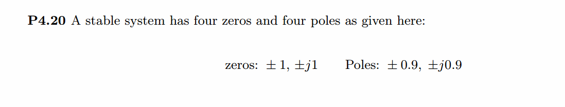
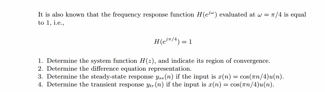
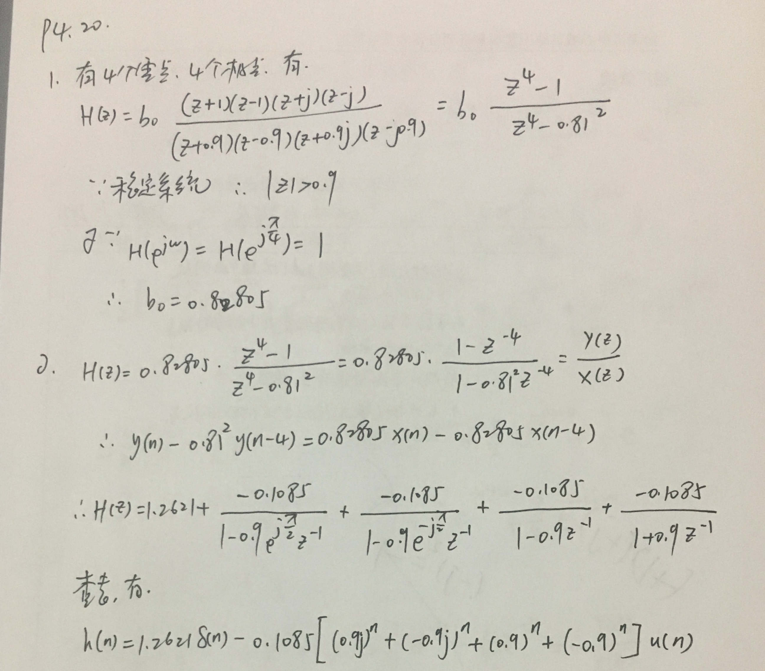
《DSP using MATLAB》Problem 4.20

代码：

%% ------------------------------------------------------------------------
%%            Output Info about this m-file
fprintf('\n***********************************************************\n');
fprintf('        <DSP using MATLAB> Problem 4.20 \n\n');

banner();
%% ------------------------------------------------------------------------

% ----------------------------------------------------
%               1        H1(z)
% ----------------------------------------------------

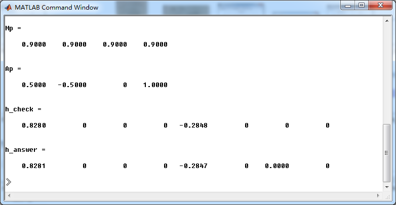
b = [1, 0, 0, 0, -1]*0.82805;
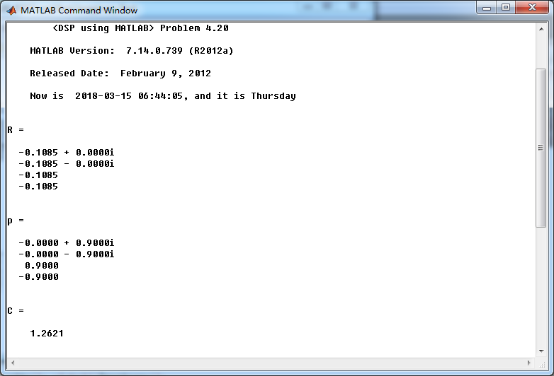
a = [1, 0, 0, 0, -0.81*0.81];               %  

[R, p, C] = residuez(b,a)

Mp = (abs(p))'
Ap = (angle(p))'/pi

%% ------------------------------------------------------
%%   START a    determine H(z) and sketch
%% ------------------------------------------------------
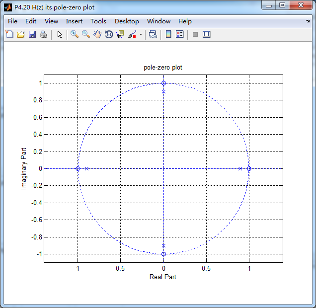
figure('NumberTitle', 'off', 'Name', 'P4.20 H(z) its pole-zero plot')
set(gcf,'Color','white');
zplane(b,a);
title('pole-zero plot'); grid on;

%% ----------------------------------------------
%%    END
%% ----------------------------------------------

% ------------------------------------
%                  h(n)
% ------------------------------------

[delta, n] = impseq(0, 0, 7);
h_check = filter(b, a, delta)                                             % check sequence

h_answer = 1.2621*impseq(0,0,7) ...
            - 0.1085*(0.9*j).^n.*stepseq(0,0,7) - 0.1085*(-0.9*j).^n.*stepseq(0,0,7) ...
            - 0.1085*(0.9).^n.*stepseq(0,0,7) - 0.1085*(-0.9).^n.*stepseq(0,0,7)         % answer sequence

%% --------------------------------------------------------------
%%    START    b   |H|   <H
%%    3rd form of freqz
%% --------------------------------------------------------------
w = [-500:1:500]*pi/500;     H = freqz(b,a,w);
%[H,w] = freqz(b,a,200,'whole');                 % 3rd form of freqz

magH  = abs(H);  angH  = angle(H);  realH  = real(H);  imagH  = imag(H);

%% ================================================
%%              START H's  mag ang real imag
%% ================================================
figure('NumberTitle', 'off', 'Name', 'P4.20  DTFT and Real Imaginary Part ');
set(gcf,'Color','white');
subplot(2,2,1); plot(w/pi,magH); grid on;  %axis([0,1,0,1.5]);
title('Magnitude Response');
xlabel('frequency in \pi units'); ylabel('Magnitude  |H|');
subplot(2,2,3); plot(w/pi, angH/pi); grid on; % axis([-1,1,-1,1]);
title('Phase Response');
xlabel('frequency in \pi units'); ylabel('Radians/\pi');

subplot('2,2,2'); plot(w/pi, realH); grid on;
title('Real Part');
xlabel('frequency in \pi units'); ylabel('Real');
subplot('2,2,4'); plot(w/pi, imagH); grid on;
title('Imaginary Part');
xlabel('frequency in \pi units'); ylabel('Imaginary');
%% ==================================================
%%             END H's  mag ang real imag
%% ==================================================

%% =========================================================
%%        Steady-State and Transient Response
%% =========================================================
bx = [1, -sqrt(2)/2]; ax = [1, -sqrt(2), 1];

by = 0.82805*conv(b, bx)
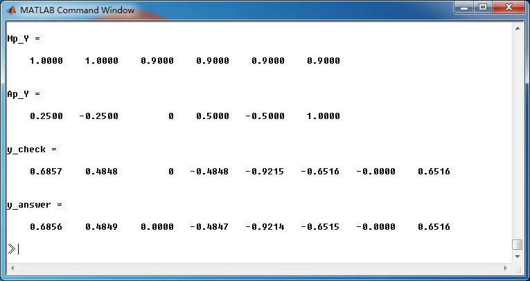
ay = conv(a, ax)

[R, p, C] = residuez(by, ay)

Mp_Y = (abs(p))'
Ap_Y = (angle(p))'/pi

%% ------------------------------------------------------
%%   START a    determine Y(z) and sketch
%% ------------------------------------------------------
figure('NumberTitle', 'off', 'Name', 'P4.20 Y(z) its pole-zero plot')
set(gcf,'Color','white');
zplane(by, ay);
title('pole-zero plot'); grid on;

% ------------------------------------
%                  y(n)
% ------------------------------------

LENGTH = 50;

[delta, n] = impseq(0, 0, LENGTH-1);
y_check = filter(by, ay, delta);                                             % check sequence

y_answer = ( 2*0.414.*(cos(pi*n/4)) - 0.029*(0.9).^n ...
           + (-2*0.0356*(0.9).^n.*cos(pi*n/2) - 2*0.0625*(0.9).^n.*sin(pi*n/2) ...
           - 0.0422*(-0.9).^n ) ) .* stepseq(0,0,LENGTH-1);

yss = 2*0.414.*(cos(pi*n/4)) .* stepseq(0,0,LENGTH-1);
yts = - 0.029*(0.9).^n ...
           + (-2*0.0356*(0.9).^n.*cos(pi*n/2) - 2*0.0625*(0.9).^n.*sin(pi*n/2) ...
           - 0.0422*(-0.9).^n ) .* stepseq(0,0,LENGTH-1);

figure('NumberTitle', 'off', 'Name', 'P4.20  Yss and Yts ');
set(gcf,'Color','white');
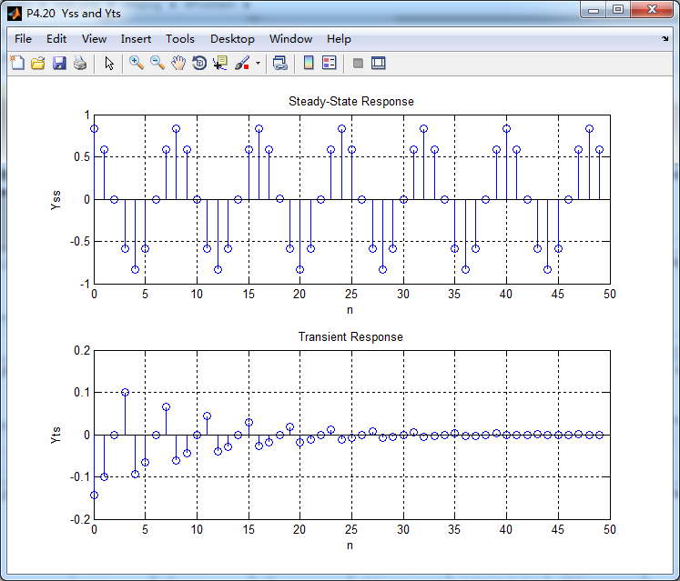
subplot(2,1,1); stem(n, yss); grid on;  %axis([0,1,0,1.5]);
title('Steady-State Response');
xlabel('n'); ylabel('Yss');
subplot(2,1,2); stem(n, yts); grid on; % axis([-1,1,-1,1]);
title('Transient Response');
xlabel('n'); ylabel('Yts');

figure('NumberTitle', 'off', 'Name', 'P4.20  Y(n) ');
set(gcf,'Color','white');
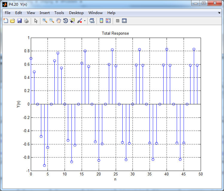
subplot(1,1,1); stem(n, y_answer); grid on;  %axis([0,1,0,1.5]);
title('Total Response');
xlabel('n'); ylabel('Y(n)');

　　运行结果：

系统函数的零极点图如下，4个极点都位于单位圆内。

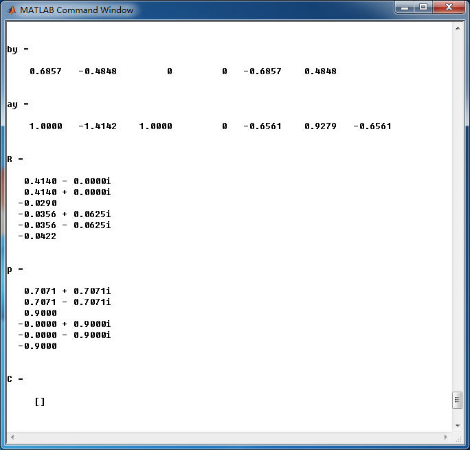
全部输出的z变换，Y（z）的零极点图如下，单位圆上的极点和稳态输出有关，单位圆内部的极点和暂态输出有关。

这里显示输出的前50个元素，下面是全输出：

稳态输出和暂态输出如下图：