第二节，TensorFlow 使用前馈神经网络实现手写数字识别

一 感知器

感知器学习笔记：https://blog.csdn.net/liyuanbhu/article/details/51622695

感知器（Perceptron）是二分类的线性分类模型，其输入为实例的特征向量，输出为实例的类别，取+1和-1。这种算法的局限性很大：

• 只能将数据分为 2 类;
• 数据必须是线性可分的;

虽然有这些局限，但是感知器是 ANN 和 SVM 的基础，理解了感知器的原理，对学习ANN 和 SVM 会有帮助，所以还是值得花些时间的。

感知器可以表示为 f:Rⁿ -> {-1,+1}的映射函数，其中f的形式如下：

f(x) = sign(w.x+b)

其中w,b都是n维列向量，w表示权重，b表示偏置，w.x表示w和x的内积。感知器的训练过程其实就是求解w和b的过程，正确的w和b所构成的超平面w.x + b=0恰好将两类数据点分割在这个平面的两侧。

二 神经网络

今天，使用的神经网络就是由一个个类似感知器的神经元模型叠加拼接成的。目前常用的神经元包括S型神经元，ReLU神经元，tanh神经元，Softmax神经元等等。

手写数字识别是目前在学习神经网络中普遍使用的案例。在这个案例中将的是简单的全连接网络实现手写数字识别，这个例子主要包括三个部分。

• .模型搭建；
• 确定目标函数，设置损失和梯度值；
• 选择算法，设置优化器选择合适的学习率更新权重和偏置；

MNIST数据集可以从这里下载：https://github.com/mnielsen/neural-networks-and-deep-learning，也可以使用TensorFlow提供的一个库，可以直接用来自动下载和安装MNIST：

from tensorflow.examples.tutorials.mnist import input_data

mnist = input_data.read_data_sets('MNIST-data',one_hot=True)

运行上面代码，会自动下载数据集并将文件解压到当前代码所在统计目录下的MNIST_data文件夹下。其中one_hot = True，表示将样本转换为one_hot编码。也就是二值化。

手写数字识别代码如下：

# -*- coding: utf-8 -*-
"""
Created on Sun Apr  1 19:16:15 2018

@author: Administrator
"""

'''
使用TnsorFlow实现手写数字识别
'''

import numpy as np
import matplotlib.pyplot as plt

#绘制训练集准确率，以及测试卷准确率曲线
def plot_overlay_accuracy(training_accuracy,test_accuaracy):
    '''
    test_accuracy,training_accuracy:训练集测试集准确率
    '''
    #迭代次数
    num_epochs = len(test_accuaracy)
    #获取一个figure实例
    fig = plt.figure()
    #使用面向对象的方式添加Axes实例，参数1：子图总行数 参数2：子图总列数 参数3：子图位置 
    ax = fig.add_subplot(111)
    ax.plot(np.arange(0, num_epochs),
            [accuracy*100.0 for accuracy in test_accuaracy],
            color='#2A6EA6',
            label="Accuracy on the test data")
    ax.plot(np.arange(0, num_epochs),
            [accuracy*100.0 for accuracy in training_accuracy],
            color='#FFA933',
            label="Accuracy on the training data")
    ax.grid(True)
    ax.set_xlim([0, num_epochs])
    ax.set_xlabel('Epoch')
    ax.set_ylim([90, 100])
    ax.legend(loc="lower right")              #右小角
    plt.show()

#绘制训练集代价和测试卷代价函数曲线
def plot_overlay_cost(training_cost,test_cost):
    '''
    test,reaining:训练集测试集代价  list类型
    '''
    #迭代次数
    num_epochs = len(test_cost)
    fig = plt.figure()
    ax = fig.add_subplot(111)
    ax.plot(np.arange(0, num_epochs),
            [cost for cost in test_cost],
            color='#2A6EA6',
            label="Cost on the test data")
    ax.plot(np.arange(0, num_epochs),
            [cost for cost in training_cost],
            color='#FFA933',
            label="Cost on the training data")
    ax.grid(True)
    ax.set_xlim([0, num_epochs])
    ax.set_xlabel('Epoch')
    #ax.set_ylim([0, 0.75])
    ax.legend(loc="upper right")
    plt.show()

from sklearn.metrics import classification_report
from sklearn.metrics import confusion_matrix
'''
打印图片
images：list或者tuple，每一个元素对应一张图片
title：list或者tuple，每一个元素对应一张图片的标题
h:高度的像素数
w:宽度像素数
n_row：输出行数
n_col：输出列数
'''
def plot_gallery(images,title,h,w,n_row=3,n_col=4):
    #pyplt的方式绘图 指定整个绘图对象的宽度和高度
    plt.figure(figsize=(1.8*n_col,2.4*n_row))
    plt.subplots_adjust(bottom=0,left=.01,right=.99,top=.90,hspace=.35)
    #绘制每个子图
    for i in range(n_row*n_col):
        #第i+1个子窗口 默认从1开始编号
        plt.subplot(n_row,n_col,i+1)
        #显示图片 传入height*width矩阵 https://blog.csdn.net/Eastmount/article/details/73392106?locationNum=5&fps=1
        plt.imshow(images[i].reshape((h,w)),cmap=plt.cm.gray)  #cmap Colormap 灰度
        #设置标题
        plt.title(title[i],size=12)
        plt.xticks(())
        plt.yticks(())
    plt.show()
'''
打印第i个测试样本对应的标题
Y_pred：测试集预测结果集合 (分类标签集合)
Y_test: 测试集真实结果集合 (分类标签集合)
target_names:分类每个标签对应的名称
i:第i个样本
'''
def title(Y_pred,Y_test,target_names,i):
    pred_name = target_names[Y_pred[i]].rsplit(' ',1)[-1]
    true_name = target_names[Y_test[i]].rsplit(' ',1)[-1]
    return 'predicted:%s\ntrue:    %s' %(pred_name,true_name)

import tensorflow as tf

#设置tensorflow对GPU使用按需分配
config = tf.ConfigProto()
config.gpu_options.allow_growth = True

sess = tf.InteractiveSession(config=config)

'''
一 导入数据
'''
from tensorflow.examples.tutorials.mnist import input_data

mnist = input_data.read_data_sets('MNIST-data',one_hot=True)

print(type(mnist)) #<class 'tensorflow.contrib.learn.python.learn.datasets.base.Datasets'>

print('Training data shape:',mnist.train.images.shape)           #Training data shape: (55000, 784)
print('Test data shape:',mnist.test.images.shape)                #Test data shape: (10000, 784)
print('Validation data shape:',mnist.validation.images.shape)    #Validation data shape: (5000, 784)
print('Training label shape:',mnist.train.labels.shape)          #Training label shape: (55000, 10)

'''
二 搭建前馈神经网络模型 搭建一个包含输入层分别为 784,1024,10个神经元的神经网络
'''

#初始化权值和偏重
def weight_variable(shape):
    #使用正太分布初始化权值
    initial = tf.truncated_normal(shape,stddev=0.1)    #标准差为0.1
    return tf.Variable(initial)

def bias_variable(shape):
    initial = tf.constant(0.1,shape=shape)
    return tf.Variable(initial)

#input layer None表示张量第一维度可以是任意长度的
x_ = tf.placeholder(tf.float32,shape=[None,784])
y_ = tf.placeholder(tf.float32,shape=[None,10])

#隐藏层
w_h = weight_variable([784,1024])
b_h = bias_variable([1024])
hidden = tf.nn.relu(tf.matmul(x_,w_h) + b_h)

#输出层
w_o = weight_variable([1024,10])
b_o = bias_variable([10])
output = tf.nn.softmax(tf.matmul(hidden,w_o) + b_o)

'''
三 设置对数似然损失函数
'''
#代价函数 J =-(Σy.logaL)/n    .表示逐元素乘
cost = tf.reduce_mean(-tf.reduce_sum(y_*tf.log(output),axis=1))

'''
四 求解
'''
train = tf.train.AdamOptimizer(0.001).minimize(cost)

#预测结果评估
#tf.argmax(output,1)  按行统计最大值得索引
correct = tf.equal(tf.argmax(output,1),tf.argmax(y_,1))       #返回一个数组 表示统计预测正确或者错误
accuracy = tf.reduce_mean(tf.cast(correct,tf.float32))   #求准确率

#创建list 保存每一迭代的结果
training_accuracy_list = []
test_accuracy_list = []
training_cost_list=[]
test_cost_list=[]

#使用会话执行图
sess.run(tf.global_variables_initializer())   #初始化变量
#开始迭代 使用Adam优化的随机梯度下降法
for i in range(5000):    #一个epoch需要迭代次数计算公式：测试集长度 / batch_size
    x_batch,y_batch = mnist.train.next_batch(batch_size = 64)
    #开始训练
    train.run(feed_dict={x_:x_batch,y_:y_batch})
    if (i+1)%200 == 0:
         #输出训练集准确率
        #training_accuracy = accuracy.eval(feed_dict={x_:mnist.train.images,y_:mnist.train.labels})
        training_accuracy,training_cost = sess.run([accuracy,cost],feed_dict={x_:mnist.train.images,y_:mnist.train.labels})
        training_accuracy_list.append(training_accuracy)
        training_cost_list.append(training_cost)
        print('{0}:Training set accuracy {1},cost {2}.'.format(i+1,training_accuracy,training_cost))
        #输出测试机准确率
        #test_accuracy = accuracy.eval(feed_dict={x_:mnist.test.images,y_:mnist.test.labels})
        test_accuracy,test_cost = sess.run([accuracy,cost],feed_dict={x_:mnist.test.images,y_:mnist.test.labels})
        test_accuracy_list.append(test_accuracy)
        test_cost_list.append(test_cost)
        print('{0}:Test set accuracy {1},cost {2}.'.format(i+1,test_accuracy,test_cost))
#绘制曲线图
plot_overlay_cost(training_cost_list,test_cost_list)
plot_overlay_accuracy(training_accuracy_list,test_accuracy_list)

#取24个样本，可视化显示预测效果
x_batch,y_batch = mnist.test.next_batch(batch_size = 24)
#获取x_batch图像对象的数字标签
y_test = np.argmax(y_batch,1)
#获取预测结果
y_pred = np.argmax(output.eval(feed_dict={x_:x_batch,y_:y_batch}),1)

#显示与分类标签0-9对应的名词
target_names = ['number 0','number 1','number 2','number 3','number 4','number 5','number 6','number 7','number 8','number 9']
#需要测试的真实的标签和预测作为比较 显示主要的分类指标，返回每个类标签的精确、召回率及F1值
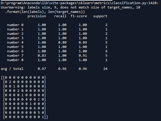
print(classification_report(y_test,y_pred,target_names = target_names))
#建立一个n*n 分别对应每一组真实的和预测的值 用于呈现一种可视化效果
print(confusion_matrix(y_test,y_pred,labels = range(len(target_names))))

#标题
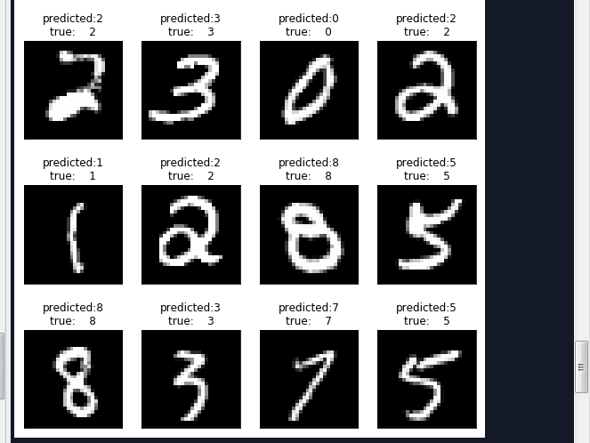
prediction_titles = [title(y_pred,y_test,target_names,i) for i in range(y_pred.shape[0])]
#打印图片
plot_gallery(x_batch,prediction_titles,28,28,6,4)

运行结果如下：

在上一个程序中有一个很明显的缺陷，我们的神经网络的层数是固定的，如果有多层的话，我们需要一一定义每一层，这样就会很麻烦，下面通过定义一个类来实现上面程序的功能。

# -*- coding: utf-8 -*-
"""
Created on Mon Apr  2 10:32:10 2018

@author: Administrator
"""

'''
定义一个network类，实现全连接网络
'''

import matplotlib.pyplot as plt

'''
打印图片
images：list或者tuple，每一个元素对应一张图片
title：list或者tuple，每一个元素对应一张图片的标题
h:高度的像素数
w:宽度像素数
n_row：输出行数
n_col：输出列数
'''
def plot_gallery(images,title,h,w,n_row=3,n_col=4):
    #pyplt的方式绘图 指定整个绘图对象的宽度和高度
    plt.figure(figsize=(1.8*n_col,2.4*n_row))
    plt.subplots_adjust(bottom=0,left=.01,right=.99,top=.90,hspace=.35)
    #绘制每个子图
    for i in range(n_row*n_col):
        #第i+1个子窗口 默认从1开始编号
        plt.subplot(n_row,n_col,i+1)
        #显示图片 传入height*width矩阵 https://blog.csdn.net/Eastmount/article/details/73392106?locationNum=5&fps=1
        plt.imshow(images[i].reshape((h,w)),cmap=plt.cm.gray)  #cmap Colormap 灰度
        #设置标题
        plt.title(title[i],size=12)
        plt.xticks(())
        plt.yticks(())
    plt.show()

'''
打印第i个测试样本对应的标题
Y_pred：测试集预测结果集合 (分类标签集合)
Y_test: 测试集真是结果集合 (分类标签集合)
target_names:分类每个标签对应的名称
i:第i个样本
'''
def title(Y_pred,Y_test,target_names,i):
    pred_name = target_names[Y_pred[i]].rsplit(' ',1)[-1]
    true_name = target_names[Y_test[i]].rsplit(' ',1)[-1]
    return 'predicted:%s\ntrue:    %s' %(pred_name,true_name)

import tensorflow as tf
import numpy as np
import random
'''
导入数据
'''
from tensorflow.examples.tutorials.mnist import input_data

mnist = input_data.read_data_sets('MNIST-data',one_hot=True)

print(type(mnist)) #<class 'tensorflow.contrib.learn.python.learn.datasets.base.Datasets'>

print('Training data shape:',mnist.train.images.shape)           #Training data shape: (55000, 784)
print('Test data shape:',mnist.test.images.shape)                #Test data shape: (10000, 784)
print('Validation data shape:',mnist.validation.images.shape)    #Validation data shape: (5000, 784)
print('Training label shape:',mnist.train.labels.shape)          #Training label shape: (55000, 10)

class network(object):
    '''
    全连接神经网络
    '''
    def __init__(self,sizes):
        '''
        注意程序中op变量只需要初始化一遍就可以，在fit()中初始化
        sizes：list传入每层神经元个数
        '''
        #保存参数
        self.__sizes = sizes
        #神经网络每一层的神经元个数数组类型
        self.sizes = tf.placeholder(tf.int64,shape=[1,len(sizes)])
        #计算神经网络层数 包括输入层
        self.num_layer = tf.size(self.sizes)
        #随机初始化权重  第i层和i+1层之间的权重向量
        self.weights = [self.weight_variable(shape=(x,y)) for x,y in  zip(sizes[:-1],sizes[1:])]
        #随机初始化偏置  第i层的偏置向量  i=1...num_layers  注意不可以设置shape=(x,1)
        self.biases = [self.bias_variable(shape=[x,]) for x in sizes[1:]] 

        #输入样本和输出类别变量
        self.x_ = tf.placeholder(tf.float32,shape=[None,sizes[0]])
        self.y_ = tf.placeholder(tf.float32,shape=[None,sizes[-1]])

        #设置tensorflow对GPU使用按需分配
        config = tf.ConfigProto()
        config.gpu_options.allow_growth = True
        self.sess = tf.InteractiveSession(config=config)

    def weight_variable(self,shape):
        '''
        初始化权值
        '''
        #使用截断式正太分布初始化权值   截断式即在正态分布基础上加以限制，以使生产的数据在一定范围上
        initial = tf.truncated_normal(shape,mean=0.0,stddev= 1.0/shape[0])    #方差为1/nin
        return tf.Variable(initial)

    def bias_variable(self,shape):
        '''
        #初始化偏重
        '''
        initial =  tf.truncated_normal(shape,mean=0.0,stddev= 1.0/shape[0])    #方差为1/nin
        return tf.Variable(initial)

    def feedforward(self,x):
        '''
        构建阶段：前向反馈
        x:变量op,tf.placeholder()类型变量
        返回一个op
        '''
        #计算隐藏层
        output = x
        for i in range(len(self.__sizes)-1):
            b = self.biases[i]
            w = self.weights[i]
            if i != len(self.__sizes)-2 :
                output =  tf.nn.relu(tf.matmul(output,w) + b)
            else:
                output = tf.nn.softmax(tf.matmul(output,w) + b)
        return output

    def fit(self,training_x,training_y,learning_rate=0.001,batch_size=64,epochs=10):
         '''
         训练神经网络
         x：训练集样本
         y:训练集样本对应的标签
         learning_rate：学习率
         batch_size:批量大小
         epochs：迭代轮数
         '''
         #计算输出层
         output = self.feedforward(self.x_)

         #代价函数 J =-(Σy.logaL)/n    .表示逐元素乘
         cost = tf.reduce_mean( -tf.reduce_sum(self.y_*tf.log(output),axis = 1))

         #求解
         train = tf.train.AdamOptimizer(learning_rate).minimize(cost)

         #使用会话执行图     

         #初始化变量 必须在train之后
         self.sess.run(tf.global_variables_initializer())  

         #训练集长度
         n = training_x.shape[0]         

         #开始迭代 使用Adam优化的随机梯度下降法
         for i in range(epochs):
              # 预取图像和label并随机打乱
              random.shuffle([training_x,training_y])
              x_batches = [training_x[k:k+batch_size] for k in range(0,n,batch_size)]
              y_batches = [training_y[k:k+batch_size] for k in range(0,n,batch_size)]

              #开始训练
              for x_batch,y_batch in zip(x_batches,y_batches):
                  train.run(feed_dict={self.x_:x_batch,self.y_:y_batch})   

              #计算每一轮迭代后的误差 并打印
              train_cost = cost.eval(feed_dict={self.x_:training_x,self.y_:training_y})
              print('Epoch {0} Training set cost {1}:'.format(i,train_cost))

    def predict(self,test_x):
        '''
        对输入test_x样本进行预测
        '''
        output = self.feedforward(self.x_)
        #使用会话执行图
        return output.eval(feed_dict={self.x_:test_x})

    def accuracy(self,x,y):
        '''
        返回值准确率
        x:测试样本集合
        y:测试类别集合
        '''
        output = self.feedforward(self.x_)
        correct = tf.equal(tf.argmax(output,1),tf.argmax(self.y_,1))       #返回一个数组 表示统计预测正确或者错误
        accuracy = tf.reduce_mean(tf.cast(correct,tf.float32))             #求准确率
        #使用会话执行图
        return accuracy.eval(feed_dict={self.x_:x,self.y_:y})

    def cost(self,x,y):
        '''
        计算代价值
        '''
        #计算输出层
        output = self.feedforward(self.x_)
        #代价函数 J =-(Σy.logaL)/n    .表示逐元素乘
        cost = tf.reduce_mean(-tf.reduce_sum(self.y_*tf.log(output),axis=1))
        #使用会话执行图
        return cost.eval(feed_dict={self.x_:x,self.y_:y})

#开始测试
nn = network([784,1024,10])
nn.fit(mnist.train.images,mnist.train.labels,0.0001,64,10)
weights = nn.sess.run(nn.weights)
print('输出权重维数：')
for weight in weights:
    print(weight.shape)
print('输出偏置维数：')
biases = nn.sess.run(nn.biases)
for biase in biases:
    print(biase.shape)
print('准确率:',nn.accuracy(mnist.test.images,mnist.test.labels))

#取24个样本，可视化显示预测效果
x_batch,y_batch = mnist.test.next_batch(batch_size = 24)
#获取x_batch图像对象的数字标签
y_test = np.argmax(y_batch,1)
#获取预测结果
y_pred = np.argmax(nn.predict(x_batch),1)

#显示与分类标签0-9对应的名词
target_names = ['number 0','number 1','number 2','number 3','number 4','number 5','number 6','number 7','number 8','number 9']

#标题
prediction_titles = [title(y_pred,y_test,target_names,i) for i in range(y_pred.shape[0])]
#打印图片
plot_gallery(x_batch,prediction_titles,28,28,6,4)

运行结果如下：