《DSP using MATLAB》Problem 7.13

代码：

%% ++++++++++++++++++++++++++++++++++++++++++++++++++++++++++++++++++++++++++++++++
%%            Output Info about this m-file
fprintf('\n***********************************************************\n');
fprintf('        <DSP using MATLAB> Problem 7.13 \n\n');

banner();
%% ++++++++++++++++++++++++++++++++++++++++++++++++++++++++++++++++++++++++++++++++

% bandstop
wp1 = 0.25*pi; ws1 = 0.35*pi; ws2=0.65*pi; wp2=0.75*pi; delta1 = 0.025; delta2 = 0.005;
tr_width = min(ws1-wp1, wp2-ws2);
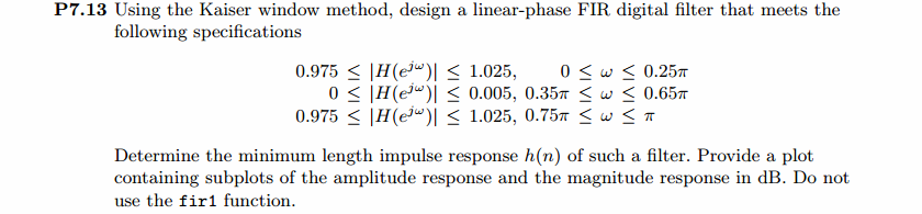
f = [wp1, ws1, ws2, wp2]/pi;

[Rp, As] = delta2db(delta1, delta2)

M = ceil((As-7.95)/(2.285*tr_width)) + 1;                 % Kaiser Window
if As > 21 || As < 50
	beta = 0.5842*(As-21)^0.4 + 0.07886*(As-21);
else
	beta = 0.1102*(As-8.7);
end

fprintf('\nKaiser Window method, Filter Length: M = %d. beta = %.4f\n', M, beta);

n = [0:1:M-1]; wc1 = (ws1+wp1)/2; wc2 = (ws2+wp2)/2;

%wc = (ws + wp)/2,                    % ideal LPF cutoff frequency

hd = ideal_lp(wc1, M) + ideal_lp(pi, M) - ideal_lp(wc2, M);
w_kai = (kaiser(M, beta))';  h = hd .* w_kai;
[db, mag, pha, grd, w] = freqz_m(h, [1]);  delta_w = 2*pi/1000;
[Hr,ww,P,L] = ampl_res(h);

Rp = -(min(db(1 :1: floor(wp1/delta_w)+1)));                     % Actual Passband Ripple
fprintf('\nActual Passband Ripple is %.4f dB.\n', Rp);

As = -round(max(db(ws1/delta_w+1 : 1 : ws2/delta_w )));   % Min Stopband attenuation
fprintf('\nMin Stopband attenuation is %.4f dB.\n', As);

[delta1, delta2] = db2delta(Rp, As)

%% ----------------------------------
%%      Increse M
%% ----------------------------------
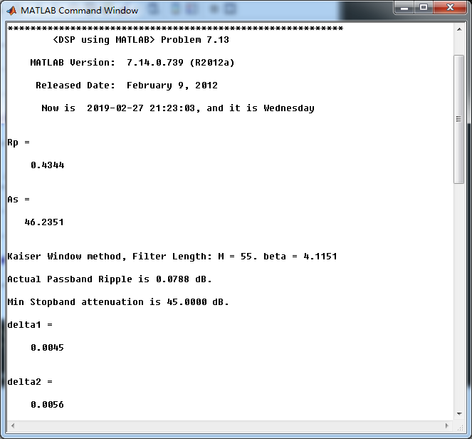
M = M+2
hd = ideal_lp(wc1, M) + ideal_lp(pi, M) - ideal_lp(wc2, M);
w_kai = (kaiser(M, beta))';  h = hd .* w_kai;
[db, mag, pha, grd, w] = freqz_m(h, [1]);  delta_w = 2*pi/1000;
[Hr,ww,P,L] = ampl_res(h);

Rp = -(min(db(1 :1: floor(wp1/delta_w)+1)));               % Actual Passband Ripple
fprintf('\nActual Passband Ripple is %.4f dB.\n', Rp);

As = -round(max(db(ws1/delta_w+1 : 1 : ws2/delta_w )));   % Min Stopband attenuation
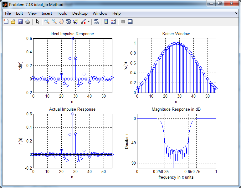
fprintf('\nMin Stopband attenuation is %.4f dB.\n', As);

[delta1, delta2] = db2delta(Rp, As)

n = [0:1:M-1];

% Plot

figure('NumberTitle', 'off', 'Name', 'Problem 7.13 ideal_lp Method')
set(gcf,'Color','white'); 

subplot(2,2,1); stem(n, hd); axis([0 M-1 -0.2 0.6]); grid on;
xlabel('n'); ylabel('hd(n)'); title('Ideal Impulse Response');

subplot(2,2,2); stem(n, w_kai); axis([0 M-1 0 1.1]); grid on;
xlabel('n'); ylabel('w(n)'); title('Kaiser Window');

subplot(2,2,3); stem(n, h); axis([0 M-1 -0.2 0.6]); grid on;
xlabel('n'); ylabel('h(n)'); title('Actual Impulse Response');

subplot(2,2,4); plot(w/pi, db); axis([0 1 -100 10]); grid on;
set(gca,'YTickMode','manual','YTick',[-90,-49,0]);
set(gca,'YTickLabelMode','manual','YTickLabel',['90';'49';' 0']);
set(gca,'XTickMode','manual','XTick',[0,f,1]);
xlabel('frequency in \pi units'); ylabel('Decibels'); title('Magnitude Response in dB');

figure('NumberTitle', 'off', 'Name', 'Problem 7.13 h(n) ideal_lp Method')
set(gcf,'Color','white'); 

subplot(2,2,1); plot(w/pi, db); grid on; axis([0 2 -100 10]);
xlabel('frequency in \pi units'); ylabel('Decibels'); title('Magnitude Response in dB');
set(gca,'YTickMode','manual','YTick',[-90,-49,0])
set(gca,'YTickLabelMode','manual','YTickLabel',['90';'49';' 0']);
set(gca,'XTickMode','manual','XTick',[0,f,1+f,2]);

subplot(2,2,3); plot(w/pi, mag); grid on; %axis([0 2 -100 10]);
xlabel('frequency in \pi units'); ylabel('Absolute'); title('Magnitude Response in absolute');
set(gca,'XTickMode','manual','XTick',[0,f,1+f,2]);
set(gca,'YTickMode','manual','YTick',[0.0,0.5,1.0])

subplot(2,2,2); plot(w/pi, pha); grid on; %axis([0 1 -100 10]);
xlabel('frequency in \pi units'); ylabel('Rad'); title('Phase Response in Radians');
subplot(2,2,4); plot(w/pi, grd*pi/180);  grid on; %axis([0 1 -100 10]);
xlabel('frequency in \pi units'); ylabel('Rad'); title('Group Delay');

figure('NumberTitle', 'off', 'Name', 'Problem 7.13 h(n)')
set(gcf,'Color','white'); 

plot(ww/pi, Hr); grid on; %axis([0 1 -100 10]);
xlabel('frequency in \pi units'); ylabel('Hr'); title('Amplitude Response');
set(gca,'YTickMode','manual','YTick',[-delta2,0,delta2,1 - delta1,1, 1 + delta1])
%set(gca,'YTickLabelMode','manual','YTickLabel',['90';'45';' 0']);
set(gca,'XTickMode','manual','XTick',[0,f,2]);

%% +++++++++++++++++++++++++++++++++++++++++
%%          fir1 function method
%% +++++++++++++++++++++++++++++++++++++++++
f = [wp1, ws1, ws2, wp2]/pi;
m = [1 0 1];
ripple = [0.025 0.005 0.025];
[N, wc, beta, ftype] = kaiserord(f,m,ripple);
fprintf('\n------------ kaiserord function: START---------------\n');
fprintf('\n--------- results used by fir1 function ---------\n');
N
wc
beta
ftype
fprintf('------------- kaiserord function: FINISH---------------\n');

%h_check = fir1(M-1, [wc1 wc2]/pi, 'stop', window(@kaiser, M));
%h_check = fir1(N, wc, ftype, window(@kaiser, N+1));
h_check = fir1(N, wc, ftype, kaiser(N+1, beta));

[db, mag, pha, grd, w] = freqz_m(h_check, [1]);
[Hr,ww,P,L] = ampl_res(h_check);

Rp = -(min(db(1 :1: floor(wp1/delta_w)+1)));              % Actual Passband Ripple
fprintf('\nActual Passband Ripple is %.4f dB.\n', Rp);

As = -round(max(db(ws1/delta_w+1 : 1 : ws2/delta_w )));   % Min Stopband attenuation
fprintf('\nMin Stopband attenuation is %.4f dB.\n', As);

%% ----------------------------------
%%            Increse N
%% ----------------------------------
N = N+2
h_check = fir1(N, wc, ftype, kaiser(N+1, beta));

[db, mag, pha, grd, w] = freqz_m(h_check, [1]);
[Hr,ww,P,L] = ampl_res(h_check);

As = -round(max(db(ws1/delta_w+1 : 1 : ws2/delta_w )));   % Min Stopband attenuation
fprintf('\nMin Stopband attenuation is %.4f dB.\n', As);

figure('NumberTitle', 'off', 'Name', 'Problem 7.13 fir1 Method')
set(gcf,'Color','white'); 

subplot(2,2,1); stem(n, hd); axis([0 M-1 -0.2 0.6]); grid on;
xlabel('n'); ylabel('hd(n)'); title('Ideal Impulse Response');

subplot(2,2,2); stem(n, w_kai); axis([0 M-1 0 1.1]); grid on;
xlabel('n'); ylabel('w(n)'); title('Kaiser Window');

subplot(2,2,3); stem([0:N], h_check); axis([0 M -0.2 0.7]); grid on;
xlabel('n'); ylabel('h\_check(n)'); title('Actual Impulse Response');

subplot(2,2,4); plot(w/pi, db); axis([0 1 -100 10]); grid on;
set(gca,'YTickMode','manual','YTick',[-90,-49,0])
set(gca,'YTickLabelMode','manual','YTickLabel',['90';'49';' 0']);
set(gca,'XTickMode','manual','XTick',[0,f,1]);
xlabel('frequency in \pi units'); ylabel('Decibels'); title('Magnitude Response in dB');

figure('NumberTitle', 'off', 'Name', 'Problem 7.13 h(n) fir1 Method')
set(gcf,'Color','white'); 

subplot(2,2,1); plot(w/pi, db); grid on; axis([0 2 -100 10]);
xlabel('frequency in \pi units'); ylabel('Decibels'); title('Magnitude Response in dB');
set(gca,'YTickMode','manual','YTick',[-90,-49,0])
set(gca,'YTickLabelMode','manual','YTickLabel',['90';'49';' 0']);
set(gca,'XTickMode','manual','XTick',[0,f,1+f,2]);

subplot(2,2,3); plot(w/pi, mag); grid on; %axis([0 1 -100 10]);
xlabel('frequency in \pi units'); ylabel('Absolute'); title('Magnitude Response in absolute');
set(gca,'XTickMode','manual','XTick',[0,f,1+f,2]);
set(gca,'YTickMode','manual','YTick',[0.0,0.5,1.0])

subplot(2,2,2); plot(w/pi, pha); grid on; %axis([0 1 -100 10]);
xlabel('frequency in \pi units'); ylabel('Rad'); title('Phase Response in Radians');
subplot(2,2,4); plot(w/pi, grd*pi/180);  grid on; %axis([0 1 -100 10]);
xlabel('frequency in \pi units'); ylabel('Rad'); title('Group Delay');

　　运行结果：

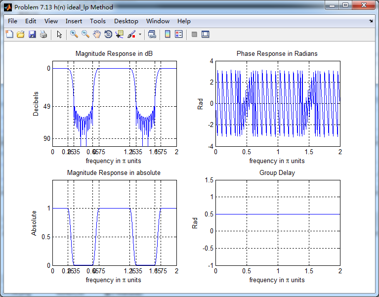
最小阻带衰减设计是46.2351dB，kaiser窗长度M=57时满足要求。

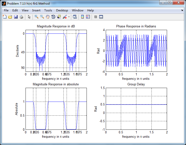
利用Kaiser窗得到的脉冲响应，计算其幅度响应（dB和Absolute单位）、相位响应和群延迟响应。

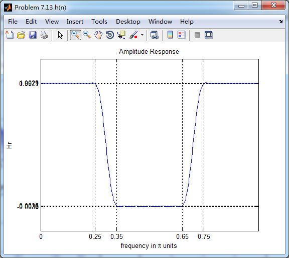
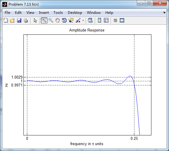
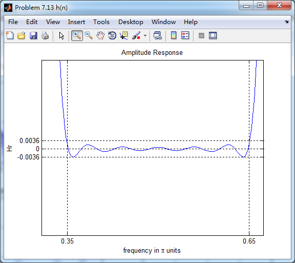
振幅响应

通带部分

阻带部分

利用fir1函数得到脉冲响应，和前面进行对比

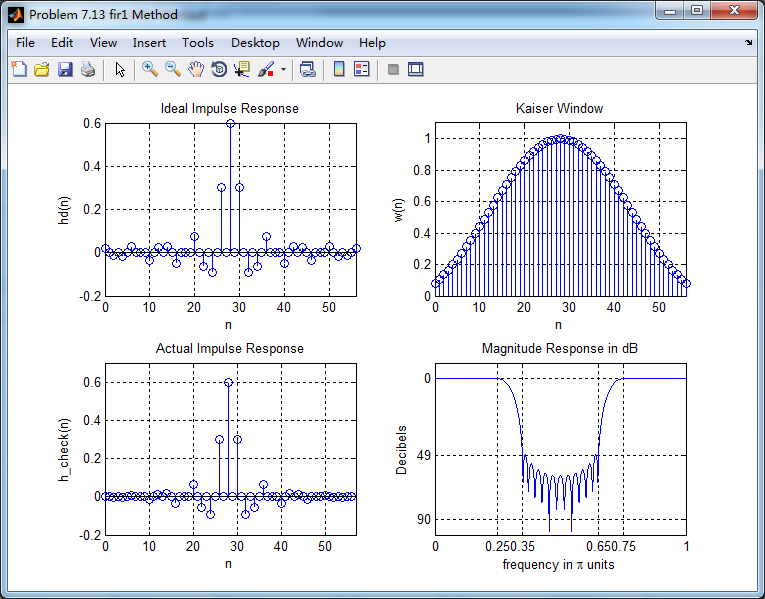
两种方法，区别不大。