《DSP using MATLAB》Problem 3.3

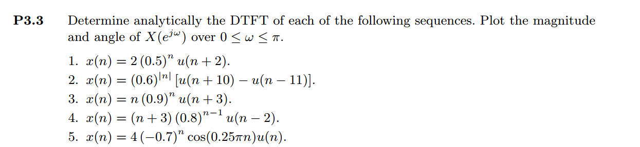
按照题目的意思需要利用DTFT的性质，得到序列的DTFT结果（公式表示），本人数学功底太差，就不写了，直接用

书中的方法计算并画图。

代码：

%% ------------------------------------------------------------------------
%%            Output Info about this m-file
fprintf('\n***********************************************************\n');
fprintf('        <DSP using MATLAB> Problem 3.3 \n\n');

banner();
%% ------------------------------------------------------------------------

% ----------------------------------
%            x1(n)
% ----------------------------------
n1_start = -3; n1_end = 13;
n1 = [n1_start : n1_end]; 

x1 = (2 * 0.5.^ (n1)) .* stepseq(-2, n1_start, n1_end); 

figure('NumberTitle', 'off', 'Name', 'Problem 3.3 x1(n)');
set(gcf,'Color','white');
stem(n1, x1);
xlabel('n'); ylabel('x1');
title('x1(n) sequence'); grid on;

M = 500;
k = [-M:M];        % [-pi, pi]
%k = [0:M];        % [0, pi]
w = (pi/M) * k;

[X1] = dtft(x1, n1, w);                            

magX1 = abs(X1); angX1 = angle(X1); realX1 = real(X1); imagX1 = imag(X1);

figure('NumberTitle', 'off', 'Name', 'Problem 3.3 DTFT of x1(n)');;
set(gcf,'Color','white');
subplot(2,1,1); plot(w/pi, magX1); grid on;
title('Magnitude Part');
xlabel('frequency in \pi units'); ylabel('Magnitude');
subplot(2,1,2); plot(w/pi, angX1); grid on;
title('Angle Part');
xlabel('frequency in \pi units'); ylabel('Radians');

X1_chk = 8*exp(j*2*w) + 4*exp(j*w) + 2 ./ (1-0.5*exp(-j*w));
magX1_chk = abs(X1_chk); angX1_chk = angle(X1_chk); realX1_chk = real(X1_chk); imagX1_chk = imag(X1_chk);

figure('NumberTitle', 'off', 'Name', 'Problem 3.3 X1(w) by formular');;
set(gcf,'Color','white');
subplot(2,1,1); plot(w/pi, magX1_chk); grid on;
title('Magnitude Part');
xlabel('frequency in \pi units'); ylabel('Magnitude');
subplot(2,1,2); plot(w/pi, angX1_chk); grid on;
title('Angle Part');
xlabel('frequency in \pi units'); ylabel('Radians');

% -------------------------------------
%            x2(n)
% -------------------------------------
n2_start = -9; n2_end = 15;
n2 = [n2_start : n2_end]; 

x2 = (0.6 .^ (abs(n2))) .* (stepseq(-10, n2_start, n2_end) - stepseq(11, n2_start, n2_end)); 

figure('NumberTitle', 'off', 'Name', 'Problem 3.3 x2(n)');
set(gcf,'Color','white');
stem(n2, x2);
xlabel('n'); ylabel('x2');
title('x2(n) sequence'); grid on;

M = 500;
k = [-M:M];        % [-pi, pi]
%k = [0:M];        % [0, pi]
w = (pi/M) * k;

[X2] = dtft(x2, n2, w);                            

magX2 = abs(X2); angX2 = angle(X2); realX2 = real(X2); imagX2 = imag(X2);

figure('NumberTitle', 'off', 'Name', 'Problem 3.3 DTFT of x2(n)');;
set(gcf,'Color','white');
subplot(2,1,1); plot(w/pi, magX2); grid on;
title('Magnitude Part');
xlabel('frequency in \pi units'); ylabel('Magnitude');
subplot(2,1,2); plot(w/pi, angX2); grid on;
title('Angle Part');
xlabel('frequency in \pi units'); ylabel('Radians');

% -------------------------------------
%            x3(n)
% -------------------------------------
n3_start = -3; n3_end = 10;
n3 = [n3_start : n3_end]; 

x3 = ( n3 .* (0.9 .^ (n3))) .* stepseq(-3, n3_start, n3_end); 

figure('NumberTitle', 'off', 'Name', 'Problem 3.3 x3(n)');
set(gcf,'Color','white');
stem(n3, x3);
xlabel('n'); ylabel('x3');
title('x3(n) sequence'); grid on;

M = 500;
k = [-M:M];        % [-pi, pi]
%k = [0:M];        % [0, pi]
w = (pi/M) * k;

[X3] = dtft(x3, n3, w);                            

magX3 = abs(X3); angX3 = angle(X3); realX3= real(X3); imagX3 = imag(X3);

figure('NumberTitle', 'off', 'Name', 'Problem 3.3 DTFT of x3(n)');;
set(gcf,'Color','white');
subplot(2,1,1); plot(w/pi, magX3); grid on;
title('Magnitude Part');
xlabel('frequency in \pi units'); ylabel('Magnitude');
subplot(2,1,2); plot(w/pi, angX3); grid on;
title('Angle Part');
xlabel('frequency in \pi units'); ylabel('Radians');

% -------------------------------------
%            x4(n)
% -------------------------------------
n4_start = 0; n4_end = 50;
n4 = [n4_start : n4_end]; 

x4 = (n4 + 3) .* (0.8 .^ (n4-1)) .* stepseq(2, n4_start, n4_end); 

figure('NumberTitle', 'off', 'Name', 'Problem 3.3 x4(n)');
set(gcf,'Color','white');
stem(n4, x4, 'r', 'filled');
xlabel('n'); ylabel('x4');
title('x4(n) sequence'); grid on;

M = 500;
k = [-M:M];        % [-pi, pi]
%k = [0:M];        % [0, pi]
w = (pi/M) * k;

[X4] = dtft(x4, n4, w);                            

magX4 = abs(X4); angX4 = angle(X4); realX4= real(X4); imagX4 = imag(X4);

figure('NumberTitle', 'off', 'Name', 'Problem 3.3 DTFT of x4(n)');;
set(gcf,'Color','white');
subplot(2,1,1); plot(w/pi, magX4); grid on;
title('Magnitude Part');
xlabel('frequency in \pi units'); ylabel('Magnitude');
subplot(2,1,2); plot(w/pi, angX4); grid on;
title('Angle Part');
xlabel('frequency in \pi units'); ylabel('Radians');

% -------------------------------------
%            x5(n)
% -------------------------------------
n5_start = 0; n5_end = 30;
n5 = [n5_start : n5_end]; 

x5 = 4 * (-7 .^ (n5)) .* cos(0.25*pi*n5) .* stepseq(0, n5_start, n5_end); 

figure('NumberTitle', 'off', 'Name', 'Problem 3.3 x5(n)');
set(gcf,'Color','white');
stem(n5, x5, 'r', 'filled');
xlabel('n'); ylabel('x5');
title('x5(n) sequence'); grid on;

M = 500;
k = [-M:M];        % [-pi, pi]
%k = [0:M];        % [0, pi]
w = (pi/M) * k;

[X5] = dtft(x5, n5, w);                            

magX5 = abs(X5); angX5 = angle(X5); realX5= real(X5); imagX5 = imag(X5);

figure('NumberTitle', 'off', 'Name', 'Problem 3.3 DTFT of x5(n)');
set(gcf,'Color','white');
subplot(2,1,1); plot(w/pi, magX5); grid on;
title('Magnitude Part');
xlabel('frequency in \pi units'); ylabel('Magnitude');
subplot(2,1,2); plot(w/pi, angX5); grid on;
title('Angle Part');
xlabel('frequency in \pi units'); ylabel('Radians');

　　运行结果：

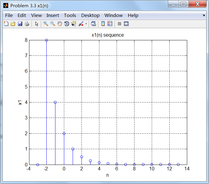
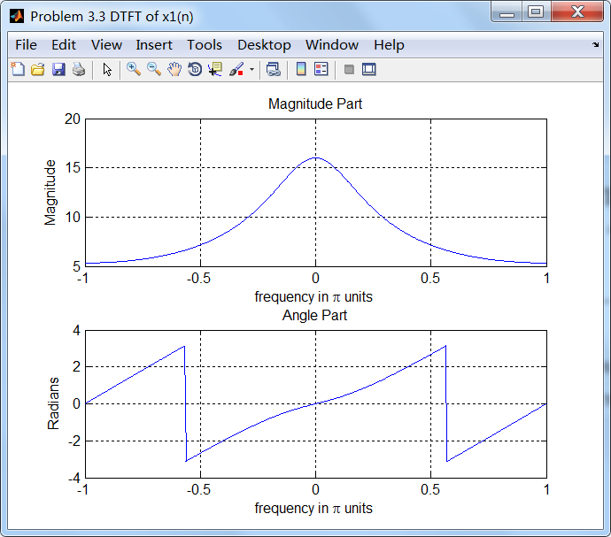
1、原始序列及其DTFT

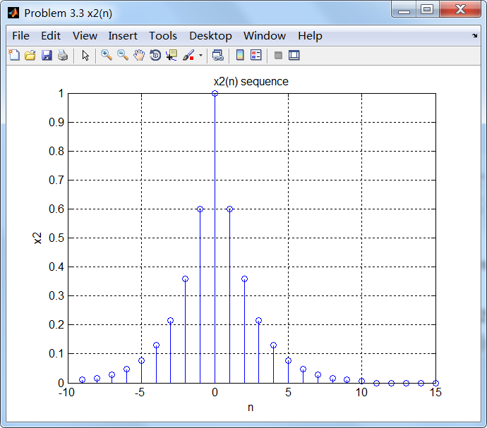
2、

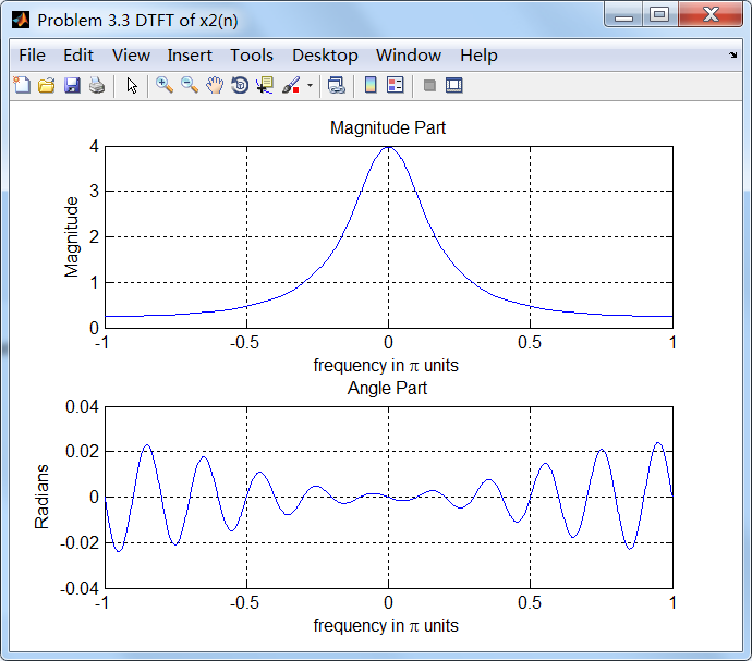
3、

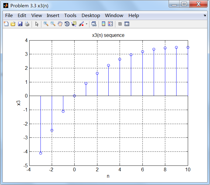
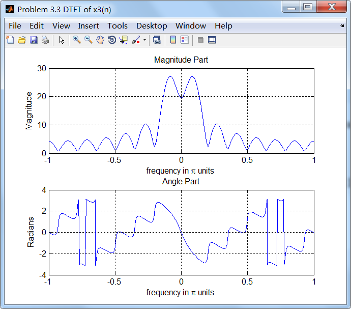
4、

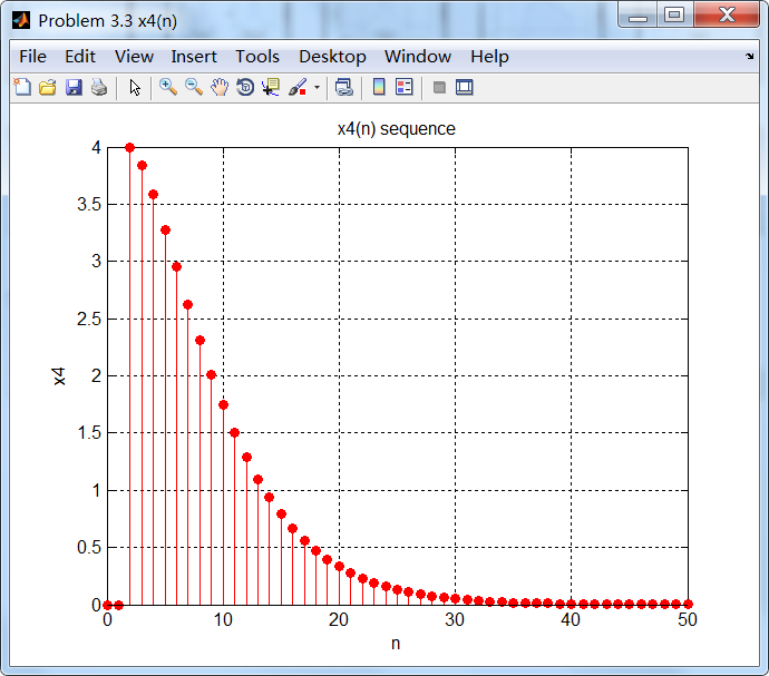
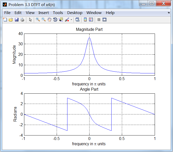
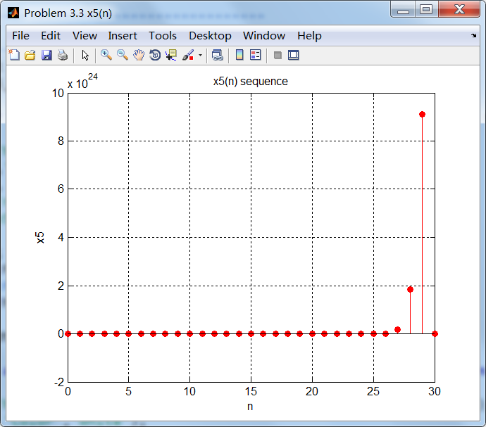
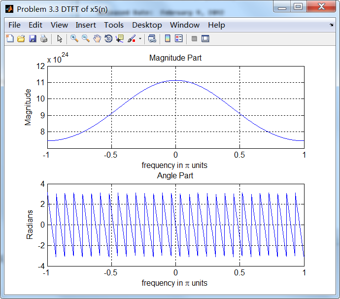
5、