Stanford coursera Andrew Ng 机器学习课程编程作业（Exercise 2）及总结

Exercise 1：Linear Regression---实现一个线性回归

关于如何实现一个线性回归，请参考：实现一个线性回归

Exercise 2：Logistic Regression---实现一个逻辑回归

问题描述：用逻辑回归根据学生的考试成绩来判断该学生是否可以入学。

这里的训练数据(training instance)是学生的两次考试成绩，以及TA是否能够入学的决定（y=0表示成绩不合格，不予录取；y=1表示录取）

因此，需要根据trainging set 训练出一个classification model。然后，拿着这个classification model 来评估新学生能否入学。

训练数据的成绩样例如下：第一列表示第一次考试成绩，第二列表示第二次考试成绩，第三列表示入学结果（0--不能入学，1--可以入学）

34.62365962451697, 78.0246928153624,  0
30.28671076822607, 43.89499752400101, 0
35.84740876993872, 72.90219802708364, 0
60.18259938620976, 86.30855209546826, 1
....
....
....

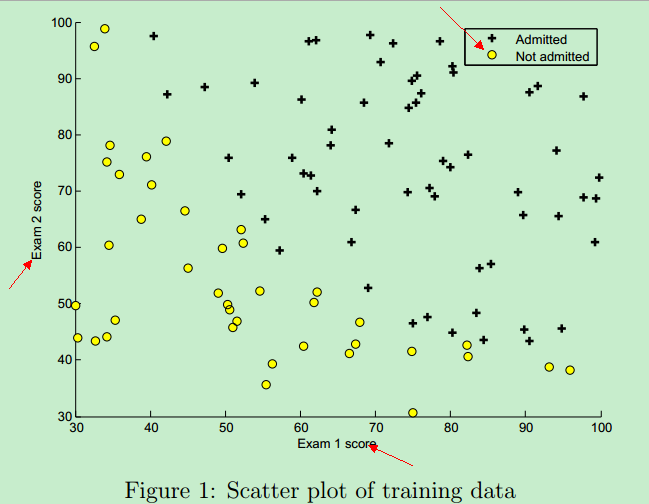
训练数据图形表示 如下：橫坐标是第一次考试的成绩，纵坐标是第二次考试的成绩，右上角的 + 表示允许入学，圆圈表示不允许入学。（分数决定命运，太悲惨了！）

该训练数据的图形 可以通过Matlab plotData函数画出来,它调用Matlab中的plot函数和find函数，Matlab代码实现如下：

function plotData(X, y)
%PLOTDATA Plots the data points X and y into a new figure
%   PLOTDATA(x,y) plots the data points with + for the positive examples
%   and o for the negative examples. X is assumed to be a Mx2 matrix.
% Create New Figure

figure; hold on;

% ====================== YOUR CODE HERE ======================
% Instructions: Plot the positive and negative examples on a
%               2D plot, using the option 'k+' for the positive
%               examples and 'ko' for the negative examples.
%

pos = find(y==);
neg = find(y==);
plot(X(pos, ), X(pos, ), 'k+', 'LineWidth', , 'MarkerSize', );
plot(X(neg, ), X(neg, ), 'ko', 'MarkerFaceColor', 'y', 'MarkerSize', );
% =========================================================================

hold off;
end

Matlab加载数据：

%% Load Data
%  The first two columns contains the exam scores and the third column
%  contains the label.

data = load('ex2data1.txt');
X = data(:, [1, 2]); y = data(:, 3);% 矩阵 X 取数据的所有行的第一列和第二列，向量 y 取数据的第三列

由上面代码可知：Matlab将文本文件中的训练数据加载到 矩阵X 和 向量 y 中

加载完数据之后，执行以下代码（调用自定义的plotData函数），将图形画出来：

plotData(X, y);

% Put some labels
hold on;
% Labels and Legend
xlabel('Exam 1 score') %标记图形的 X 轴
ylabel('Exam 2 score') %标记图形的 Y 轴

% Specified in plot order
legend('Admitted', 'Not admitted') %图形的右上角标签
hold off;

图形画出来之后，对训练数据就有了一个大体的可视化的认识了。接下来就要实现 模型了，这里需要训练一个逻辑回归模型。

①sigmoid function

对于 logistic regression而言，它针对的是 classification problem。这里只讨论二分类问题，比如上面的“根据成绩入学”，结果只有两种：y==0时，成绩未合格，不予入学；y==1时，可入学。即，y的输出要么是0，要么是1

如果采用 linear regression，它的假设函数是这样的：

假设函数的取值即可以远远大于1，也可以远远小于0，并且容易受到一些特殊样本的影响。比如在上图中，就只能约定：当假设函数大于等于0.5时；预测y==1，小于0.5时，预测y==0。

而如果引入了sigmoid function，就可以把假设函数的值域“约束”在[0, 1]之间。总之，引入sigmoid function，就能够更好的拟合分类问题中的数据，即从这个角度看：regression model 比 linear model 更合适 classification problem.

引入sigmoid后，假设函数如下：

sigmoid function 用Matlab 实现如下：

function g = sigmoid(z)
%SIGMOID Compute sigmoid functoon
%   J = SIGMOID(z) computes the sigmoid of z.

% You need to return the following variables correctly
g = zeros(size(z));

% ====================== YOUR CODE HERE ======================
% Instructions: Compute the sigmoid of each value of z (z can be a matrix,
%               vector or scalar).

g = 1./(ones(size(z)) + exp(-z)); % ‘点除’ 表示 1 除以矩阵(向量)中的每一个元素

% =============================================================

end

②模型的代价函数(cost function)

什么是代价函数呢？

把训练好的模型对新数据进行预测，那预测结果有好有坏。因此，就用cost function 来衡量预测的"准确性"。cost function越小，表示测的越准。这里的代价函数的本质是”最小二乘法“---ordinary least squares

代价函数的最原始的定义是下面的这个公式：可见，它是关于 theta 的函数。(X，y 是已知的，由training set 中的数据确定了)

那如何求解 cost function的参数 theta，从而确定J(theta)呢？有两种方法：一种是梯度下降算法(Gradient descent)，另一种是正规方程(Normal Equation)，本文只讨论Gradient descent。

而梯度下降算法，本质上是求导数(偏导数)，或者说是：方向导数。方向导数所代表的方向--梯度方向，下降得最快。

而我们知道，对于某些图形所代表的函数，它可能有很多个导数为0的点，这类函数称为非凸函数(non-convex function)；而某些函数，它只有一个全局唯一的导数为0的点，称为 convex function，比如下图：

convex function能够很好地让Gradient descent寻找全局最小值。而上图左边的non-convex就不太适用Gradient descent了。

就是因为上面这个原因，logistic regression 的 cost function被改写成了下面这个公式：

可以看出，引入log 函数（对数函数），让non-convex function 变成了 convex function

再精简一下cost function，其实它可以表示成：

J(theta)可用向量表示成：

其Matlab语言表示公式如下：

J = ( log( sigmoid(theta'*X') ) * y + log( 1-sigmoid(theta'*X') ) * (1 - y) )/(-m);

③梯度下降算法

上面已经讲到梯度下降算法本质上是求偏导数，目标就是寻找theta，使得 cost function J(theta)最小。公式如下：

上面对theta(j)求偏导数，得到的值就是梯度j，记为：grad(j)

通过线性代数中的矩阵乘法以及向量的乘法规则，可以将梯度grad表示成向量的形式：

至于如何证明的，可参考：Exercise 1：Linear Regression---实现一个线性回归

其Matlab语言表示公式如下：

grad = ( X' * ( sigmoid(X*theta)-y ) )/m; % X 为 training set 中的 feature variables, y 为training instance(训练样本的结果)结果

需要注意的是：对于logistic regression，假设函数h(x)=g(z)，即它引入了sigmoid function.

最终，Matlab中costfunction.m如下：

function [J, grad] = costFunction(theta, X, y)
%COSTFUNCTION Compute cost and gradient for logistic regression
%   J = COSTFUNCTION(theta, X, y) computes the cost of using theta as the
%   parameter for logistic regression and the gradient of the cost
%   w.r.t. to the parameters.

% Initialize some useful values
m = length(y); % number of training examples

% You need to return the following variables correctly
J = 0;
grad = zeros(size(theta));

% ====================== YOUR CODE HERE ======================
% Instructions: Compute the cost of a particular choice of theta.
%               You should set J to the cost.
%               Compute the partial derivatives and set grad to the partial
%               derivatives of the cost w.r.t. each parameter in theta
%
% Note: grad should have the same dimensions as theta
%

%J = (log(theta'*X')*y + (1-y)*log(1-theta'*X'))/(-m);
%attention matlab's usage
J = ( log( sigmoid(theta'*X') ) * y + log( 1-sigmoid(theta'*X') ) * (1 - y) )/(-m);

% theta = theta - (alpha/m)*X'*(X*theta-y);
grad = ( X' * ( sigmoid(X*theta)-y ) )/m;

% =============================================================

end

通过调用costfunction.m文件中定义的coustFunction函数，从而运行梯度下降算法找到使代价函数J(theta)最小化的 逻辑回归模型参数theta。调用costFunction函数的代码如下：

%% ============= Part 3: Optimizing using fminunc  =============
%  In this exercise, you will use a built-in function (fminunc) to find the
%  optimal parameters theta.

%  Set options for fminunc
options = optimset('GradObj', 'on', 'MaxIter', 400);

%  Run fminunc to obtain the optimal theta
%  This function will return theta and the cost
[theta, cost] = ...
    fminunc(@(t)(costFunction(t, X, y)), initial_theta, options);

从上面代码的最后一行可以看出，我们是通过 fminunc 调用 costFunction函数，来求得 theta的，而不是自己使用 Gradient descent 在for 循环求导来计算 theta。for循环中求导计算theta，可参考：Exercise 1：Linear Regression---实现一个线性回归

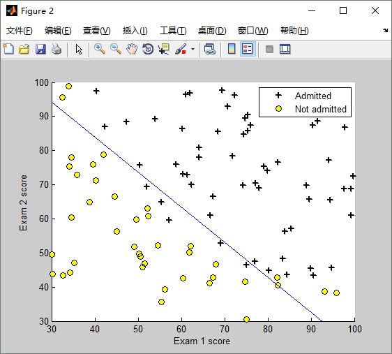
既然已经通过Gradient descent算法求得了theta，将theta代入到假设函数中，就得到了 logistic regression model，用图形表示如下：

④模型的评估（Evaluating logistic regression）

那如何估计，求得的逻辑回归模型是好还是坏呢？预测效果怎么样？因此，就需要拿一组数据测试一下，测试代码如下：

%% ============== Part 4: Predict and Accuracies ==============
%  After learning the parameters, you'll like to use it to predict the outcomes
%  on unseen data. In this part, you will use the logistic regression model
%  to predict the probability that a student with score 45 on exam 1 and
%  score 85 on exam 2 will be admitted.
%
%  Furthermore, you will compute the training and test set accuracies of
%  our model.
%
%  Your task is to complete the code in predict.m

%  Predict probability for a student with score 45 on exam 1
%  and score 85 on exam 2 

prob = sigmoid([1 45 85] * theta); %这是一组测试数据，第一次考试成绩为45，第二次成绩为85
fprintf(['For a student with scores 45 and 85, we predict an admission ' ...
         'probability of %f\n\n'], prob);

% Compute accuracy on our training set
p = predict(theta, X);% 调用predict函数测试模型

fprintf('Train Accuracy: %f\n', mean(double(p == y)) * 100);

fprintf('\nProgram paused. Press enter to continue.\n');
pause;

模型的测试结果如下：

For a student with scores 45 and 85, we predict an admission probability of 0.774323

Train Accuracy: 89.000000

那predict函数是如何实现的呢？predict.m 如下：

function p = predict(theta, X)
%PREDICT Predict whether the label is 0 or 1 using learned logistic
%regression parameters theta
%   p = PREDICT(theta, X) computes the predictions for X using a
%   threshold at 0.5 (i.e., if sigmoid(theta'*x) >= 0.5, predict 1)

m = size(X, 1); % Number of training examples

% You need to return the following variables correctly
p = zeros(m, 1);

% ====================== YOUR CODE HERE ======================
% Instructions: Complete the following code to make predictions using
%               your learned logistic regression parameters.
%               You should set p to a vector of 0's and 1's
%
p = X*theta >= 0;

% =========================================================================

end

非常简单，只有一行代码：p = X * theta >= 0，原理如下：

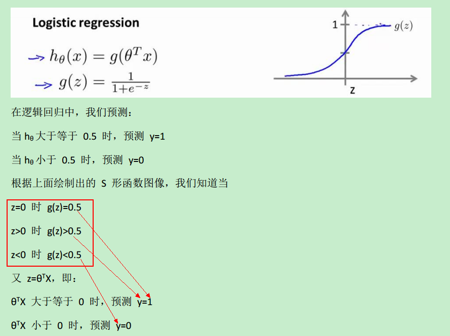
当h(x)>=0.5时，预测y==1，而h(x)>=0.5 等价于 z>=0

⑤逻辑回归的正则化（Regularized logistic regression）

为什么需要正则化？正则化就是为了解决过拟合问题(overfitting problem)。那什么又是过拟合问题呢？

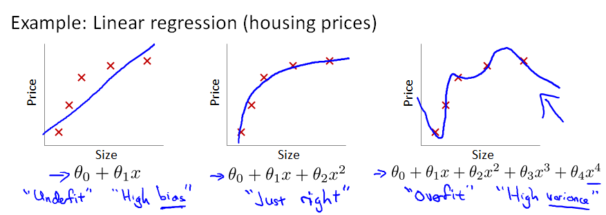
一般而言，当模型的特征(feature variables)非常多，而训练的样本数目(training set)又比较少的时候，训练得到的假设函数(hypothesis function)能够非常好地匹配training set中的数据，此时的代价函数几乎为0。下图中最右边的那个模型 就是一个过拟合的模型。

所谓过拟合，从图形上看就是：假设函数曲线完美地通过中样本中的每一个点。也许有人会说：这不正是最完美的模型吗？它完美地匹配了traing set中的每一个样本呀！

过拟合模型不好的原因是：尽管它能完美匹配traing set中的每一个样本，但它不能很好地对未知的 (新样本实例)input instance 进行预测呀！通俗地讲，就是过拟合模型的预测能力差。

因此，正则化(regularization)就出马了。

前面提到，正是因为 feature variable非常多，导致 hypothesis function 的幂次很高，hypothesis function变得很复杂(弯弯曲曲的)，从而通过穿过每一个样本点(完美匹配每个样本)。如果添加一个"正则化项"，减少 高幂次的特征变量的影响，那 hypothesis function不就变得平滑了吗？

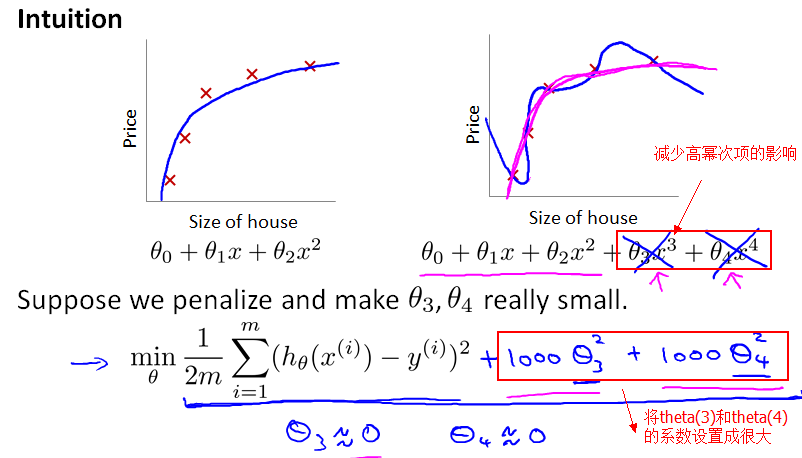
正如前面提到，梯度下降算法的目标是最小化cost function，而现在把 theta(3) 和 theta(4)的系数设置为1000，设得很大，求偏导数时，相应地得到的theta(3) 和 theta(4) 就都约等于0了。

更一般地，我们对每一个theta(j)，j>=1，进行正则化，就得到了一个如下的代价函数：其中的 lambda(λ)就称为正则化参数(regularization parameter)

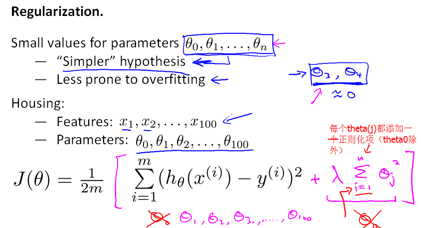
从上面的J(theta)可以看出：如果lambda(λ)=0，则表示没有使用正则化；如果lambda(λ)过大，使得模型的各个参数都变得很小，导致h(x)=theta(0)，从而造成欠拟合；如果lambda(λ)很小，则未充分起到正则化的效果。因此，lambda(λ)的值要合适。

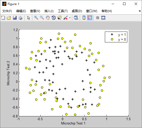
最后，我们来看一个实际的过拟合的示例，原始的训练数据如下图：

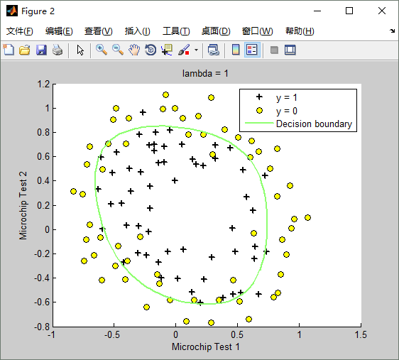
lambda(λ)==1时，训练出来的模型（hypothesis function）如下：Train Accuracy: 83.050847

lambda(λ)==0时，不使用正则化，训练出来的模型（hypothesis function）如下：Train Accuracy: 87.288136

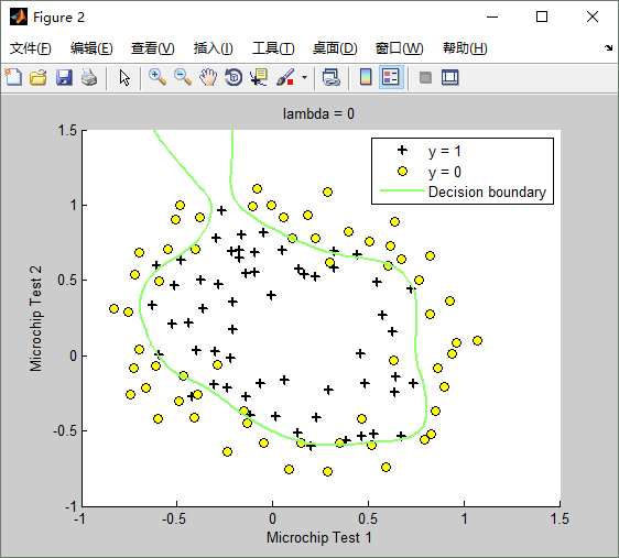
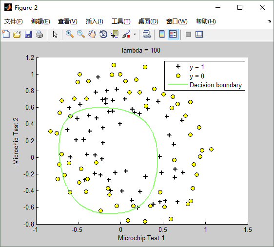
lambda(λ)==100时，训练出来的模型（hypothesis function）如下：Train Accuracy: 61.016949

Matlab正则化代价函数的实现文件costFunctionReg.m如下：

function [J, grad] = costFunctionReg(theta, X, y, lambda)
%COSTFUNCTIONREG Compute cost and gradient for logistic regression with regularization
%   J = COSTFUNCTIONREG(theta, X, y, lambda) computes the cost of using
%   theta as the parameter for regularized logistic regression and the
%   gradient of the cost w.r.t. to the parameters. 

% Initialize some useful values
m = length(y); % number of training examples

% You need to return the following variables correctly
J = 0;
grad = zeros(size(theta));

% ====================== YOUR CODE HERE ======================
% Instructions: Compute the cost of a particular choice of theta.
%               You should set J to the cost.
%               Compute the partial derivatives and set grad to the partial
%               derivatives of the cost w.r.t. each parameter in theta
%J = ( log( sigmoid(theta'*X') ) * y + log( 1-sigmoid(theta'*X') ) * (1 - y) )/(-m);
%J = ( log( sigmoid(theta'*X') ) * y + log( 1-sigmoid(theta'*X') ) * (1 - y) )/(-m) + (lambda / (2*m)) * (theta'*theta);
J = ( log( sigmoid(theta'*X') ) * y + log( 1-sigmoid(theta'*X') ) * (1 - y) )/(-m) + (lambda / (2*m)) * ( ( theta( 2:length(theta) ) )' * theta(2:length(theta)) );
%grad = ( X' * ( sigmoid(X*theta)-y ) )/m;
grad = ( X' * ( sigmoid(X*theta)-y ) )/m + ( lambda / m ) * ( [0; ones( length(theta) - 1 , 1 )].*theta );

% =============================================================

end

调用costFunctionReg.m的代码如下：

%% ============= Part 2: Regularization and Accuracies =============
%  Optional Exercise:
%  In this part, you will get to try different values of lambda and
%  see how regularization affects the decision coundart
%
%  Try the following values of lambda (0, 1, 10, 100).
%
%  How does the decision boundary change when you vary lambda? How does
%  the training set accuracy vary?
%

% Initialize fitting parameters
initial_theta = zeros(size(X, 2), 1);

% Set regularization parameter lambda to 1 (you should vary this)
lambda = 1;

% Set Options
options = optimset('GradObj', 'on', 'MaxIter', 400);

% Optimize
[theta, J, exit_flag] = ...
    fminunc(@(t)(costFunctionReg(t, X, y, lambda)), initial_theta, options);

% Plot Boundary
plotDecisionBoundary(theta, X, y);
hold on;
title(sprintf('lambda = %g', lambda))

% Labels and Legend
xlabel('Microchip Test 1')
ylabel('Microchip Test 2')

legend('y = 1', 'y = 0', 'Decision boundary')
hold off;

% Compute accuracy on our training set
p = predict(theta, X);

fprintf('Train Accuracy: %f\n', mean(double(p == y)) * 100);

⑥总结：

本文是对Stanford Machine Learning课程中的logistic regression的总结。结合课后编程习题，对logistic regression 各个知识点和编程作业中的代码、实现原理作了详细的解释。

有兴趣并且有时间学一名新技术是一件幸福的事情。

原文：http://www.cnblogs.com/hapjin/p/6078530.html