
《DSP using MATLAB》Problem 8.31

代码:
%% ------------------------------------------------------------------------

%%            Output Info about this m-file

fprintf('\n***********************************************************\n');

fprintf('        <DSP using MATLAB> Problem 8.31 \n\n');

banner();

%% ------------------------------------------------------------------------

Fp = 3.2;                    % analog passband freq in kHz   6.4 kpi

Fs = 3.8;                    % analog stopband freq in kHz   7.6 kpi

fs = 8;                      % sampling rate in kHz         16.0 kpi

% -------------------------------

%       Ω=(2/T)tan(ω/2)

%       ω=2*[atan(ΩT/2)]

% Digital Filter Specifications:

% -------------------------------

wp = 2*pi*Fp/fs                 % digital passband freq in rad     0.8pi

%wp = Fp;

ws = 2*pi*Fs/fs                 % digital stopband freq in rad     0.95pi

%ws = Fs;

Rp = 0.5;                        % passband ripple in dB

As = 45;                         % stopband attenuation in dB

Ripple = 10 ^ (-Rp/20)           % passband ripple in absolute

Attn = 10 ^ (-As/20)             % stopband attenuation in absolute

% Analog prototype specifications: Inverse Mapping for frequencies

T = 1/8000;                           % set T = 1

%fs = 1/T;

OmegaP = (2/T)*tan(wp/2)        % prototype passband freq      1.9593pi     15675pi

OmegaS = (2/T)*tan(ws/2)        % prototype stopband freq      8.089pi      64712pi

% Analog Chebyshev-1 Prototype Filter Calculation:

[cs, ds] = afd_chb1(OmegaP, OmegaS, Rp, As);

% Calculation of second-order sections:

fprintf('\n***** Cascade-form in s-plane: START *****\n');

[CS, BS, AS] = sdir2cas(cs, ds)

fprintf('\n***** Cascade-form in s-plane: END *****\n');

% Calculation of Frequency Response:

[db_s, mag_s, pha_s, ww_s] = freqs_m(cs, ds, 8*pi/T);

% --------------------------------------------------------------------

%   find exact band-edge frequencies for the given dB specifications

% --------------------------------------------------------------------

[diff_to_45dB, ind] = min(abs(db_s+45))

db_s(ind-3 : ind+3)                                     % magnitude response, dB

ww_s(ind)/(pi)          % analog frequency in kpi units

%ww_s(ind)/(2*pi)        % analog frequency in Hz units

[sA,index] = sort(abs(db_s+45));

AA_dB = db_s(index(1:8))

AB_rad = ww_s(index(1:8))/(pi)

AC_Hz = ww_s(index(1:8))/(2*pi)

% -------------------------------------------------------------------

% Calculation of Impulse Response:

[ha, x, t] = impulse(cs, ds);

% Impulse Invariance Transformation:

%[b, a] = imp_invr(cs, ds, T);

% Bilinear Transformation

[b, a] = bilinear(cs, ds, 1/T)

[C, B, A] = dir2cas(b, a)

% Calculation of Frequency Response:

[db, mag, pha, grd, ww] = freqz_m(b, a);

% --------------------------------------------------------------------

%   find exact band-edge frequencies for the given dB specifications

% --------------------------------------------------------------------

[diff_to_45dB, ind] = min(abs(db+45))

db(ind-3 : ind+3)                                     % magnitude response, dB

ww(ind)/(pi)

(2/T)*tan(ww(ind)/2)/pi

[sA,index] = sort(abs(db+45));

AA_dB = db(index(1:8))'

AB_rad = ww(index(1:8))'/pi

AC_Hz = (2/T)*tan(ww(index(1:8))'/2)/pi

% -------------------------------------------------------------------

%% -----------------------------------------------------------------

%%                             Plot

%% -----------------------------------------------------------------

figure('NumberTitle', 'off', 'Name', 'Problem 8.31 Analog Chebyshev-I lowpass')

set(gcf,'Color','white');

M = 1.0;                          % Omega max

subplot(2,2,1); plot(ww_s/pi, mag_s);  grid on; %axis([-10, 10, 0, 1.2]);

xlabel(' Analog frequency in \piHz units'); ylabel('|H|'); title('Magnitude in Absolute');

% set(gca, 'XTickMode', 'manual', 'XTick', [-8.089, -1.9593, 0, 1.9593, 8.089]);  % T = 1

set(gca, 'XTickMode', 'manual', 'XTick', [-80000, -64712, -15675, 0, 15675, 64712, 80000]);  % T = 1/8000

set(gca, 'YTickMode', 'manual', 'YTick', [0, 0.006, 0.94, 1.0, 1.5]);

subplot(2,2,2); plot(ww_s/pi, db_s);  grid on; %axis([0, M, -50, 10]);

xlabel('Analog frequency in \piHz units'); ylabel('Decibels'); title('Magnitude in dB ');

% set(gca, 'XTickMode', 'manual', 'XTick', [-8.089, -1.9593, 0, 1.9593, 5.7, 8.089]);        % T = 1

set(gca, 'XTickMode', 'manual', 'XTick', [-80000, -64712, -15675, 0, 15675, 45696, 64712, 80000]);  % T = 1/8000

set(gca, 'YTickMode', 'manual', 'YTick', [-45, -1, 0]);

set(gca,'YTickLabelMode','manual','YTickLabel',['45';' 1';' 0']);

subplot(2,2,3); plot(ww_s/pi, pha_s/pi);  grid on; %axis([-10, 10, -1.2, 1.2]);

xlabel('Analog frequency in \piHz nuits'); ylabel('radians'); title('Phase Response');

% set(gca, 'XTickMode', 'manual', 'XTick', [-8.089, -1.9593, 0, 1.9593, 8.089]);    % T = 1

set(gca, 'XTickMode', 'manual', 'XTick', [-80000, -64712, -15675, 0, 15675, 45696, 64712, 80000]);  % T = 1/8000

set(gca, 'YTickMode', 'manual', 'YTick', [-1:0.5:1]);

subplot(2,2,4); plot(t, ha); grid on; %axis([0, 30, -0.05, 0.25]);

xlabel('time in seconds'); ylabel('ha(t)'); title('Impulse Response');

figure('NumberTitle', 'off', 'Name', 'Problem 8.31 Digital Chebyshev-I lowpass')

set(gcf,'Color','white');

M = 2;                          % Omega max

subplot(2,2,1); plot(ww/pi, mag); axis([0, M, 0, 1.2]); grid on;

xlabel(' Digital frequency in \pi units'); ylabel('|H|'); title('Magnitude Response');

set(gca, 'XTickMode', 'manual', 'XTick', [0, 0.8, 0.95, M]);

set(gca, 'YTickMode', 'manual', 'YTick', [0, 0.0056, 0.9441, 1]);

subplot(2,2,2); plot(ww/pi, pha/pi); axis([0, M, -1.1, 1.1]); grid on;

xlabel('Digital frequency in \pi nuits'); ylabel('radians in \pi units'); title('Phase Response');

set(gca, 'XTickMode', 'manual', 'XTick', [0, 0.8, 0.95, M]);

set(gca, 'YTickMode', 'manual', 'YTick', [-1:1:1]);

subplot(2,2,3); plot(ww/pi, db); axis([0, M, -80, 10]); grid on;

xlabel('Digital frequency in \pi units'); ylabel('Decibels'); title('Magnitude in dB ');

set(gca, 'XTickMode', 'manual', 'XTick', [0, 0.8, 0.93, 0.95, M]);

set(gca, 'YTickMode', 'manual', 'YTick', [-70, -45, -1, 0]);

set(gca,'YTickLabelMode','manual','YTickLabel',['70';'45';' 1';' 0']);

subplot(2,2,4); plot(ww/pi, grd); grid on; %axis([0, M, 0, 35]);

xlabel('Digital frequency in \pi units'); ylabel('Samples'); title('Group Delay');

set(gca, 'XTickMode', 'manual', 'XTick', [0, 0.8, 0.95, M]);

%set(gca, 'YTickMode', 'manual', 'YTick', [0:5:35]);

figure('NumberTitle', 'off', 'Name', 'Problem 8.31 Pole-Zero Plot')

set(gcf,'Color','white');

zplane(b,a);

title(sprintf('Pole-Zero Plot'));

%pzplotz(b,a);

% ----------------------------------------------

%       Calculation of Impulse Response

% ----------------------------------------------

figure('NumberTitle', 'off', 'Name', 'Problem 8.31 Imp & Freq Response')

set(gcf,'Color','white');

t = [0: 0.000005 : 8*0.0001]; subplot(2,1,1); impulse(cs,ds,t); grid on;   % Impulse response of the analog filter

axis([0, 8*0.0001, -1.5*10000, 2.0*10000]);hold on

n = [0:1:7*0.0001/T]; hn = filter(b,a,impseq(0,0,7*0.0001/T));           % Impulse response of the digital filter

stem(n*T,hn); xlabel('time in sec'); title (sprintf('Impulse Responses T=%2d',T));

hold off

% Calculation of Frequency Response:

[dbs, mags, phas, wws] = freqs_m(cs, ds, 8*pi/T);             % Analog frequency   s-domain

[dbz, magz, phaz, grdz, wwz] = freqz_m(b, a);                  % Digital  z-domain

%% -----------------------------------------------------------------

%%                             Plot

%% -----------------------------------------------------------------

subplot(2,1,2); plot(wws/(2*pi), mags/T, 'b+', wwz/(2*pi*T), magz, 'r'); grid on;

xlabel('frequency in Hz'); title('Magnitude Responses'); ylabel('Magnitude');

text(-0.8,0.15,'Analog filter', 'Color', 'b'); text(0.6,1.05,'Digital filter', 'Color', 'r');

%% -----------------------------------------------------------------------

%%                   MATLAB cheby1 function

%% -----------------------------------------------------------------------

% Analog Prototype Order Calculations:

ep = sqrt(10^(Rp/10)-1);           % Passband Ripple Factor

A = 10^(As/20);                    % Stopband Attenuation Factor

OmegaC = OmegaP;                   % Analog Chebyshev-1 prototype cutoff freq

OmegaR = OmegaS/OmegaP;            % Analog prototype Transition ratio

g = sqrt(A*A-1)/ep;                % Analog prototype Intermediate cal

N  = ceil(log10(g+sqrt(g*g-1))/log10(OmegaR+sqrt(OmegaR*OmegaR-1)));

fprintf('\n\n ********** Chebyshev-I Filter Order = %3.0f  \n', N)

% Digital Chebyshev-1 Filter Design:

wn = wp/pi;                        % Digital Chebyshev-1 cutoff freq in pi units

[b, a] = cheby1(N, Rp, wn)

[C, B, A] = dir2cas(b, a)

% Calculation of Frequency Response:

[db, mag, pha, grd, ww] = freqz_m(b, a);

% --------------------------------------------------------------------

%   find exact band-edge frequencies for the given dB specifications

% --------------------------------------------------------------------

[diff_to_45dB, ind] = min(abs(db+45))

db(ind-3 : ind+3)                                     % magnitude response, dB

ww(ind)/(pi)

(2/T)*tan(ww(ind)/2)/pi

[sA,index] = sort(abs(db+45));

AA_dB = db(index(1:8))'

AB_rad = ww(index(1:8))'/pi

AC_Hz = (2/T)*tan(ww(index(1:8))'/2)/pi

% -------------------------------------------------------------------

%% -----------------------------------------------------------------

%%                             Plot

%% -----------------------------------------------------------------

figure('NumberTitle', 'off', 'Name', 'Problem 8.31 Digital Chebyshev-I lowpass by cheby1 function')

set(gcf,'Color','white');

M = 2;                          % Omega max

subplot(2,2,1); plot(ww/pi, mag); axis([0, M, 0, 1.2]); grid on;

xlabel('Digital frequency in \pi units'); ylabel('|H|'); title('Magnitude Response');

set(gca, 'XTickMode', 'manual', 'XTick', [0, 0.8, 0.95, M]);

set(gca, 'YTickMode', 'manual', 'YTick', [0, 0.0056, 0.9441, 1]);

subplot(2,2,2); plot(ww/pi, pha/pi); axis([0, M, -1.1, 1.1]); grid on;

xlabel('Digital frequency in \pi nuits'); ylabel('radians in \pi units'); title('Phase Response');

set(gca, 'XTickMode', 'manual', 'XTick', [0, 0.8, 0.95, M]);

set(gca, 'YTickMode', 'manual', 'YTick', [-1:1:1]);

subplot(2,2,3); plot(ww/pi, db); axis([0, M, -100, 10]); grid on;

xlabel('Digital frequency in \pi units'); ylabel('Decibels'); title('Magnitude in dB ');

set(gca, 'XTickMode', 'manual', 'XTick', [0, 0.8, 0.93, 0.95, M]);

set(gca, 'YTickMode', 'manual', 'YTick', [-60, -45, -1, 0]);

set(gca,'YTickLabelMode','manual','YTickLabel',['60';'45';' 1';' 0']);

subplot(2,2,4); plot(ww/pi, grd); grid on; %axis([0, M, 0, 35]);

xlabel('Digital frequency in \pi units'); ylabel('Samples'); title('Group Delay');

set(gca, 'XTickMode', 'manual', 'XTick', [0, 0.8, 0.95, M]);

%set(gca, 'YTickMode', 'manual', 'YTick', [0:5:35]);

figure('NumberTitle', 'off', 'Name', 'Problem 8.31 Pole-Zero Plot')

set(gcf,'Color','white');

zplane(b,a);

title(sprintf('Pole-Zero Plot'));

%pzplotz(b,a);

% ----------------------------------------------

%       Calculation of Impulse Response

% ----------------------------------------------

figure('NumberTitle', 'off', 'Name', 'Problem 8.31 Imp & Freq Response')

set(gcf,'Color','white');

t = [0: 0.000005 : 8*0.0001]; subplot(2,1,1); impulse(cs,ds,t); grid on;   % Impulse response of the analog filter

axis([0, 8*0.0001, -1.5*10000, 2.0*10000]);hold on

n = [0:1:7*0.0001/T]; hn = filter(b,a,impseq(0,0,7*0.0001/T));           % Impulse response of the digital filter

stem(n*T,hn); xlabel('time in sec'); title (sprintf('Impulse Responses T=%2d',T));

hold off

% Calculation of Frequency Response:

[dbs, mags, phas, wws] = freqs_m(cs, ds, 8*pi/T);             % Analog frequency   s-domain

[dbz, magz, phaz, grdz, wwz] = freqz_m(b, a);                  % Digital  z-domain

%% -----------------------------------------------------------------

%%                             Plot

%% -----------------------------------------------------------------

subplot(2,1,2); plot(wws/(2*pi), mags/T, 'b+', wwz/(2*pi*T), magz, 'r'); grid on;

xlabel('frequency in Hz'); title('Magnitude Responses'); ylabel('Magnitude');

text(-0.8,0.15,'Analog filter', 'Color', 'b'); text(0.6,1.05,'Digital filter', 'Color', 'r');
运行结果:
这里放上T=1/8000sec的结果。
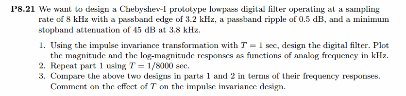
模拟chebyshev-1型低通,幅度谱、相位谱和脉冲响应
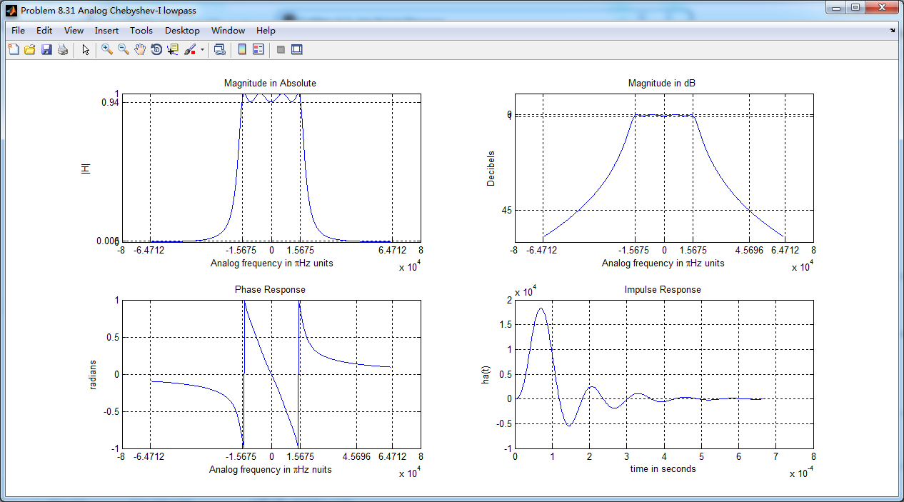
采用双线性变换法,得到数字chebyshev-1型低通滤波器,幅度谱、相位谱和群延迟响应
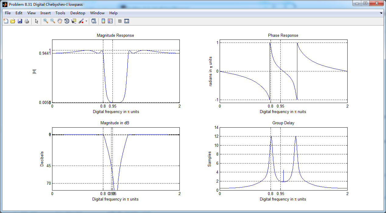
采用MATLAB自带cheby1函数得到的数字低通,其幅度谱、相位谱和群延迟

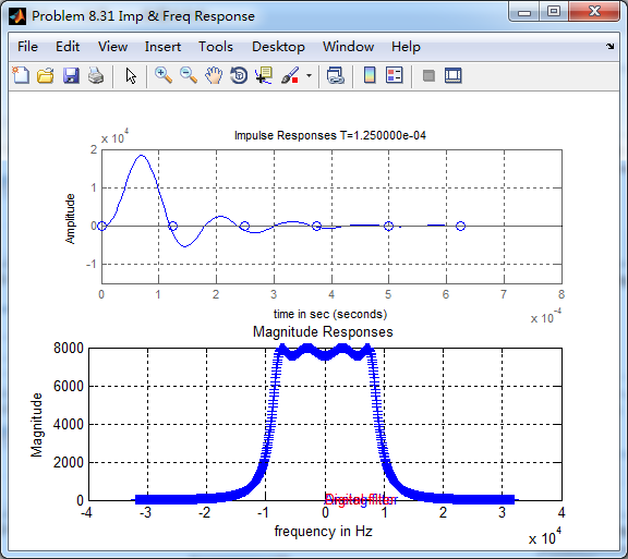
cheby1函数得到的数字低通,和相应的模拟原型的脉冲响应,二者形态不同。
《DSP using MATLAB》Problem 8.31的更多相关文章
- 《DSP using MATLAB》Problem 5.31
第3小题: 代码: %% ++++++++++++++++++++++++++++++++++++++++++++++++++++++++++++++++++++++++++++++++ %% Out ...
- 《DSP using MATLAB》Problem 7.31
参照Example7.27,因为0.1π=2πf1 f1=0.05,0.9π=2πf2 f2=0.45 所以0.1π≤ω≤0.9π,0.05≤|H|≤0.45 代码: %% +++++++++ ...
- 《DSP using MATLAB》Problem 7.26
注意:高通的线性相位FIR滤波器,不能是第2类,所以其长度必须为奇数.这里取M=31,过渡带里采样值抄书上的. 代码: %% +++++++++++++++++++++++++++++++++++++ ...
- 《DSP using MATLAB》Problem 7.25
代码: %% ++++++++++++++++++++++++++++++++++++++++++++++++++++++++++++++++++++++++++++++++ %% Output In ...
- 《DSP using MATLAB》Problem 7.24
又到清明时节,…… 注意:带阻滤波器不能用第2类线性相位滤波器实现,我们采用第1类,长度为基数,选M=61 代码: %% +++++++++++++++++++++++++++++++++++++++ ...
- 《DSP using MATLAB》Problem 6.12
代码: %% ++++++++++++++++++++++++++++++++++++++++++++++++++++++++++++++++++++++++++++++++ %% Output In ...
- 《DSP using MATLAB》Problem 6.10
代码: %% ++++++++++++++++++++++++++++++++++++++++++++++++++++++++++++++++++++++++++++++++ %% Output In ...
- 《DSP using MATLAB》Problem 2.7
1.代码: function [xe,xo,m] = evenodd_cv(x,n) % % Complex signal decomposition into even and odd parts ...
- 《DSP using MATLAB》Problem 2.6
1.代码 %% ------------------------------------------------------------------------ %% Output Info abou ...
随机推荐
- more指令和less指令使用的区别
more和less都是可以一页一页的翻动 more翻页的时候,显示有百分比在最下一行 less没有 more可以用来查询 空白键 (space):代表向下翻一页:Enter :代表向下翻『一行』:/字 ...
- 解决Keep-Alive 和 Close 不能使用此属性设置
http://www.hejingzong.cn/blog/viewblog_86.aspx Keep-Alive 和 Close 不能使用此属性设置 public static void SetHe ...
- range和arange
a = np.arange(12) print(a, type(a)) b = range(10) print(b, type(b)) li = list(b) print(li) 拓展: 两个参数: ...
- 实现虚拟机VMware上Linux与本机windows互相复制与粘贴的问题
解决方法:只需要在Linux系统中安装一个vmware-tools的工具 1.选择虚拟机菜单,有安装vmware tools 工具的选项 点击之后,在Linux的桌面下会出现 VMwareTools. ...
- Altera的primary register和secondary register
在Altera的一些IP文档上,提到IP的资源使用情况时,会有primary logic register和secondary logic register这样的术语. 那么什么是primary/se ...
- You can tell a lot about somebody, looking him in the eye.
You can tell a lot about somebody, looking him in the eye.注视着别人的眼睛,你能读出很多故事.
- input、textarea等输入框输入中文时,拼音在输入框内会触发input事件的问题
监听文本输入框的input事件,在拼写汉字(输入法)但汉字并未实际填充到文本框中(选词)时会触发input事件,如图: 但是在很多情况下,只需要输入到输入框的中文字符. 解决办法: 通过查阅资料得知在 ...
- for循环总结
1.冒泡排序的总结:其实这个很简单的理解,就是用数组里面的第0个元素(也就是[]里面的第一个数,按照数组的话是第一个,让他们进行挨个比较),示例: 排序前: 14 62 38 41 53 62 71 ...
- 尚学python课程---13、python基础语法
尚学python课程---13.python基础语法 一.总结 一句话总结: legend2系统使我能够快速掌握一门语法,特别有用 pass 语句:空语句:是为了保持程序结构的完整性 :作用:比如: ...
- JS 变量的数据类型转换
变量的类型转换,一般情况是JS自动转换的,但也有些时候需要手动转换. 1.其它类型转成布尔型 函数和方法的区别 Boolean(a) //函数是可以独立使用的 document.write(a) ...