[Scikit-learn] 1.1 Generalized Linear Models - Logistic regression & Softmax

二分类：Logistic regression

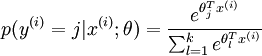
多分类：Softmax分类函数

对于损失函数，我们求其最小值，

对于似然函数，我们求其最大值。

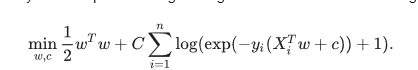
Logistic是loss function，即：

　　在逻辑回归中，选择了 “对数似然损失函数”，L(Y,P(Y|X)) = -logP(Y|X)。

　　对似然函数求最大值，其实就是对对数似然损失函数求最小值。

Logistic regression, despite its name, is a linear model for classification rather than regression.

（但非回归，其实是分类，通过后验概率比较，那么如何求MLE就是收敛的核心问题）

逻辑回归与正则化

As an optimization problem, binary class L2 penalized logistic regression minimizes the following cost function:

Similarly, L1 regularized logistic regression solves the following optimization problem

Optimal Solvers

逻辑回归提供的四种 “渐近算法”

The solvers implemented in the class LogisticRegression are “liblinear”, “newton-cg”, “lbfgs” and “sag”: （收敛算法，例如梯度下降等）

“lbfgs” 和 “newton-cg” 只支持L2罚项，并且对于一些高维数据收敛非常快。L1罚项产生稀疏预测的权重。

“liblinear” 使用了基于Liblinear的坐标下降法(CD)。

　　对于L1罚项， sklearn.svm.l1_min_c 允许计算C的下界以获得一个非”null” 的 模型（所有特征权重为0）。

　　这依赖于非常棒的一个库 LIBLINEAR library，用在scikit-learn中。 然而，CD算法在liblinear中的实现无法学习一个真正的多维（多类）的模型；反而，最优问题被分解为 “one-vs-rest” 多个二分类问题来解决多分类。

　　由于底层是这样实现的，所以使用了该库的 LogisticRegression 类就可以作为多类分类器了。

特点分析

LogisticRegression 使用 “lbfgs” 或者 “newton-cg” 程序 来设置 multi_class 为 “”，则该类学习 了一个真正的多类逻辑回归模型，也就是说这种概率估计应该比默认 “one-vs-rest” 设置要更加准确。

但是 “lbfgs”, “newton-cg” 和 “sag” 程序无法优化 含L1罚项的模型，所以”multinomial” 的设置无法学习稀疏模型。

“sag” 程序使用了随机平均梯度下降（ Stochastic Average Gradient descent）。它无法解决多分类问题，而且对于含L2罚项的模型有局限性。 然而在超大数据集下计算要比其他程序快很多，当样本数量和特征数量都非常大的时候。

In a nutshell, one may choose the solver with the following rules:

Case	Solver
Small dataset or L1 penalty	“liblinear”
Multinomial loss or large dataset	“lbfgs”, “sag” or “newton-cg”
Very Large dataset	“sag”

注：

For large dataset, you may also consider using SGDClassifier(Stochastic Gradient Descent) with ‘log’ loss.

Goto: [Scikit-learn] 1.5 Generalized Linear Models - Stochastic Gradient Descent

数学原理

---

原理大放送

Ref: 机器学习算法与Python实践之（七）逻辑回归（Logistic Regression）

Ref: 对于logistic函数的交叉熵损失函数

(a) 概率模型 - Logistic Regression

将 “参数”与“变量”的关系 转化为了概率关系；σ是sigmoid函数。

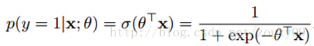
本质就是：转化为概率的思维模式；转化的方式有很多种，这种相对最好。

LogisticRegression 就是一个被logistic方程归一化后的线性回归。

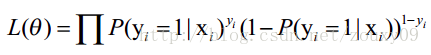
(b) 代价函数 - MLE

LogisticRegression最基本的学习算法是最大似然。

似然作为 "cost function"

【交叉熵】

这个似然的角度得出的上述公式结论，其实也就是交叉熵：goto 简单的交叉熵损失函数，你真的懂了吗？

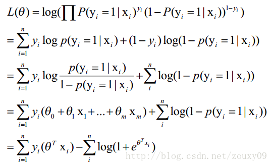
(c) 优化似然

Log 似然作为 "cost function" 会容易计算一些。

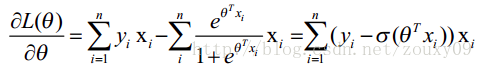
(d) 渐近求解

导数 = 0： 但貌似不好求，便有了 solver (“liblinear”, “newton-cg”, “lbfgs” and “sag”)。

其中：solver = “sag”时，参考：[Scikit-learn] 1.5 Generalized Linear Models - SGD for Classification中的

clf = SGDClassifier(loss="log", alpha=0.01, n_iter=200, fit_intercept=True)

一个 loss function 对应一堆 solvers；

一个 solver 对应一堆 loss functions；

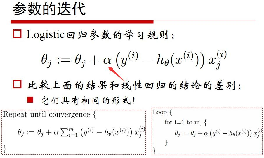
逼近的过程形式化为迭代公式：

Logistic 代码实现

逻辑实现

from __future__ import print_function

import numpy as np
import matplotlib.pyplot as plt

# Define the logistic function
def logistic(z):
  return 1 / (1 + np.exp(-z))　　`

# Plot the logistic function
z = np.linspace(-6,6,100)
plt.plot(z, logistic(z), 'b-')　　// <-- 画图

plt.xlabel('$z$', fontsize=15)
plt.ylabel('$\sigma(z)$', fontsize=15)
plt.title('logistic function')
plt.grid()
plt.show()

Result: 

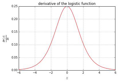
求导实现

# Define the logistic function
def logistic_derivative(z):
  return logistic(z) * (1 - logistic(z))




# Plot the derivative of the logistic function
z = np.linspace(-6,6,100)
plt.plot(z, logistic_derivative(z), 'r-')　　// <-- 画图

plt.xlabel('$z$', fontsize=15)
plt.ylabel('$\\frac{\\partial \\sigma(z)}{\\partial z}$', fontsize=15)
plt.title('derivative of the logistic function')
plt.grid()
plt.show()

Result:  

线性多分类

---

Ref: LogisticRegression（参数解密）

Logistic Regression (aka logit, MaxEnt) classifier.

多分类策略

‘multi_class’ option :

• • ‘ovr’: one-vs-rest (OvR)
  • 'multinomial': cross- entropy loss【it is supported only by the ‘lbfgs’, ‘sag’ and ‘newton-cg’ solvers.】

正则化的参数

参数 penalty

【str, ‘l1’, ‘l2’, ‘elasticnet’ or ‘none’, optional (default=’l2’)】

This class implements regularized logistic regression using the ‘liblinear’ library, ‘newton-cg’, ‘sag’ and ‘lbfgs’ solvers.

参数 solver

【str, {‘newton-cg’, ‘lbfgs’, ‘liblinear’, ‘sag’, ‘saga’}, optional (default=’liblinear’)】

It can handle both dense and sparse input. Use C-ordered arrays or CSR matrices containing 64-bit floats for optimal performance; any other input format will be converted (and copied).

• • The ‘newton-cg’, ‘sag’, and ‘lbfgs’ solvers support only L2 regularization with primal formulation.
  • The ‘liblinear’ solver supports both L1 and L2 regularization, with a dual formulation only for the L2 penalty.

参数 C

【float, default: 1.0】

Inverse of regularization strength; must be a positive float. Like in support vector machines, smaller values specify stronger regularization.

Answer: 参数越小则表明越强的正则化：正则项系数的倒数

 

参数 multi_class

【str, {‘ovr’, ‘multinomial’}, default: ‘ovr’】

Multiclass option can be either ‘ovr’ or ‘multinomial’. If the option chosen is ‘ovr’, then a binary problem is fit for each label. Else the loss minimised is the multinomial loss fit across the entire probability distribution. Works only for the ‘newton-cg’, ‘sag’ and ‘lbfgs’ solver.

New in version 0.18: Stochastic Average Gradient descent solver for ‘multinomial’ case.

正则化逻辑回归

例一：L1 Penalty and Sparsity in Logistic Regression

# 有点仅一层的logit NN的意思

"""
==============================================
L1 Penalty and Sparsity in Logistic Regression
==============================================

Comparison of the sparsity (percentage of zero coefficients) of solutions when
L1 and L2 penalty are used for different values of C. We can see that large
values of C give more freedom to the model.  Conversely, smaller values of C
constrain the model more. In the L1 penalty case, this leads to sparser
solutions.

We classify 8x8 images of digits into two classes: 0-4 against 5-9.
The visualization shows coefficients of the models for varying C.
"""

print(__doc__)

# Authors: Alexandre Gramfort <alexandre.gramfort@inria.fr>
#          Mathieu Blondel <mathieu@mblondel.org>
#          Andreas Mueller <amueller@ais.uni-bonn.de>
# License: BSD 3 clause

import numpy as np
import matplotlib.pyplot as plt

from sklearn.linear_model import LogisticRegression
from sklearn import datasets
from sklearn.preprocessing import StandardScaler

digits = datasets.load_digits()

X, y = digits.data, digits.target
X    = StandardScaler().fit_transform(X)

# 四舍五如
y = (y > 4).astype(np.int)

# Set regularization parameter
for i, C in enumerate((100, 1, 0.01)):
    # turn down tolerance for short training time
    clf_l1_LR = LogisticRegression(C=C, penalty='l1', tol=0.01)
    clf_l2_LR = LogisticRegression(C=C, penalty='l2', tol=0.01)
    clf_l1_LR.fit(X, y)
    clf_l2_LR.fit(X, y)

    coef_l1_LR = clf_l1_LR.coef_.ravel()
    coef_l2_LR = clf_l2_LR.coef_.ravel()

    # coef_l1_LR contains zeros due to the
    # L1 sparsity inducing norm

    sparsity_l1_LR = np.mean(coef_l1_LR == 0) * 100
    sparsity_l2_LR = np.mean(coef_l2_LR == 0) * 100

    print("C=%.2f" % C)
    print("Sparsity with L1 penalty: %.2f%%" % sparsity_l1_LR)
    print("score with L1 penalty: %.4f" % clf_l1_LR.score(X, y))
    print("Sparsity with L2 penalty: %.2f%%" % sparsity_l2_LR)
    print("score with L2 penalty: %.4f" % clf_l2_LR.score(X, y))

    l1_plot = plt.subplot(3, 2, 2 * i + 1)
    l2_plot = plt.subplot(3, 2, 2 * (i + 1))
    if i == 0:
        l1_plot.set_title("L1 penalty")
        l2_plot.set_title("L2 penalty")

    l1_plot.imshow(np.abs(coef_l1_LR.reshape(8, 8)), interpolation='nearest', cmap='binary', vmax=1, vmin=0)
    l2_plot.imshow(np.abs(coef_l2_LR.reshape(8, 8)), interpolation='nearest', cmap='binary', vmax=1, vmin=0)
    plt.text(-8, 3, "C = %.2f" % C)

    l1_plot.set_xticks(())
    l1_plot.set_yticks(())
    l2_plot.set_xticks(())
    l2_plot.set_yticks(())

plt.show()

Result:  

C=100.00
Sparsity with L1 penalty: 6.25%
score with L1 penalty: 0.9104
Sparsity with L2 penalty: 4.69%
score with L2 penalty: 0.9098
C=1.00
Sparsity with L1 penalty: 9.38%
score with L1 penalty: 0.9098
Sparsity with L2 penalty: 4.69%
score with L2 penalty: 0.9093
C=0.01
Sparsity with L1 penalty: 85.94%
score with L1 penalty: 0.8598
Sparsity with L2 penalty: 4.69%
score with L2 penalty: 0.8915

Jeff：如上，权重的归零化显而易见。

例二：Path with L1- Logistic Regression

print(__doc__)

# Author: Alexandre Gramfort <alexandre.gramfort@inria.fr>
# License: BSD 3 clause

from datetime import datetime
import numpy as np
import matplotlib.pyplot as plt

from sklearn import linear_model
from sklearn import datasets
from sklearn.svm import l1_min_c

iris = datasets.load_iris()
X = iris.data
y = iris.target

X = X[y != 2]
y = y[y != 2]

X -= np.mean(X, 0)

###############################################################################
# Demo path functions
cs = l1_min_c(X, y, loss='log') * np.logspace(0, 3)
# 对正则化的强度取不同值，实验各自效果

print("Computing regularization path ...")
start = datetime.now()
clf   = linear_model.LogisticRegression(C=1.0, penalty='l1', tol=1e-6)
coefs_ = []
for c in cs:
    clf.set_params(C=c)
    clf.fit(X, y)
    coefs_.append(clf.coef_.ravel().copy())
print("This took ", datetime.now() - start)

coefs_ = np.array(coefs_)
plt.plot(np.log10(cs), coefs_)
ymin, ymax = plt.ylim()
plt.xlabel('log(C)')
plt.ylabel('Coefficients')
plt.title('Logistic Regression Path')
plt.axis('tight')
plt.show()

系数的变化

coefs_
Out[30]:
array([[ 0.        ,  0.        ,  0.        ,  0.        ],
       [ 0.        ,  0.        ,  0.17813685,  0.        ],
       [ 0.        ,  0.        ,  0.3384641 ,  0.        ],
       ...,
       [ 0.        , -1.29412716,  5.71841258,  0.        ],
       [ 0.        , -1.41538897,  5.82221819,  0.        ],
       [ 0.        , -1.53535948,  5.92878532,  0.        ]])

Result:

Jeff：四个系数对应四根线，类似于trace plot，其实还是在说L1, L2的东西。

Softmax 多分类

Ref: Softmax函数解密

Ref: http://www.cnblogs.com/daniel-D/archive/2013/05/30/3109276.html

Ref: http://ufldl.stanford.edu/wiki/index.php/Softmax%E5%9B%9E%E5%BD%92

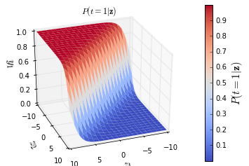
立体 sigmoid

先来个炫酷的立体sigmoid作为开场：

import numpy as np
import matplotlib.pyplot as plt
from matplotlib import cm

# Define the softmax function
def softmax(z):
    return np.exp(z) / np.sum(np.exp(z))
#--------------------------------------------------------------------------

# Plot the softmax output for 2 dimensions for both classes
# Plot the output in function of the weights
# Define a vector of weights for which we want to plot the ooutput
nb_of_zs = 200
zs = np.linspace(-10, 10, num=nb_of_zs) # input
zs_1, zs_2 = np.meshgrid(zs, zs) # generate grid
y = np.zeros((nb_of_zs, nb_of_zs, 2)) # initialize output
# Fill the output matrix for each combination of input z's
for i in range(nb_of_zs):
    for j in range(nb_of_zs):
        y[i,j,:] = softmax(np.asarray([zs_1[i,j], zs_2[i,j]]))
# Plot the cost function surfaces for both classes
fig = plt.figure()
# Plot the cost function surface for t=1
ax = fig.gca(projection='3d')
surf = ax.plot_surface(zs_1, zs_2, y[:,:,0], linewidth=0, cmap=cm.coolwarm)
ax.view_init(elev=30, azim=70)
cbar = fig.colorbar(surf)
ax.set_xlabel('$z_1$', fontsize=15)
ax.set_ylabel('$z_2$', fontsize=15)
ax.set_zlabel('$y_1$', fontsize=15)
ax.set_title ('$P(t=1|\mathbf{z})$')
cbar.ax.set_ylabel('$P(t=1|\mathbf{z})$', fontsize=15)
plt.grid()
plt.show()

Result: 

基本原理

在数字手写识别中，我们要识别的是十个类别，每次从输入层输入 28×28 个像素，输出层就可以得到本次输入可能为 0, 1, 2… 的概率。

简易版本的，看起来更直观:

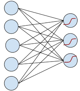
OK, 左边是输入层，输入的 x 通过中间的黑线 w (包含了 bias 项)作用下，得到 w.x, 到达右边节点， 右边节点通过红色的函数将这个值映射成一个概率，预测值就是输入概率最大的节点，这里可能的值是 {0, 1, 2}。

在实现Softmax回归时，将  用一个  的矩阵来表示会很方便，该矩阵是将  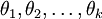按行罗列起来得到的，如下所示： (k是类别数，n是输入channel数)

在 softmax regression 中，输入的样本属于第 j 类的概率可以写成：

注意到，这个回归的参数向量减去一个常数向量，会有什么结果：

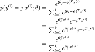
没有变化！(指数函数的无记忆性)

如果某一个向量是代价函数的极小值点，那么这个向量在减去一个任意的常数向量也是极小值点，这是因为 softmax 模型被过度参数化了。

进一步而言，如果参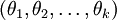数  是代价函数  的极小值点，那么  同样也是它的极小值点，其中  可以为任意向量。因此使  最小化的解不是唯一的。

（有趣的是，由于  仍然是一个凸函数，因此梯度下降时不会遇到局部最优解的问题。但是 Hessian 矩阵是奇异的/不可逆的，这会直接导致采用牛顿法优化就遇到数值计算的问题）

注意，当  时，我们总是可以将 替换为（即替换为全零向量），并且这种变换不会影响假设函数。因此我们可以去掉参数向量  （或者其他  中的任意一个）而不影响假设函数的表达能力。实际上，与其优化全部的  个参数  （其中 ），我们可以令 ，只优化剩余的  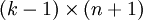个参数，这样算法依然能够正常工作。

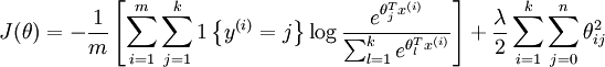
在实际应用中，为了使算法实现更简单清楚，往往保留所有参数 ，而不任意地将某一参数设置为 0。但此时我们需要对代价函数做一个改动：加入权重衰减。权重衰减可以解决 softmax 回归的参数冗余所带来的数值问题。

既然模型被过度参数化了，我们就事先确定一个参数，比如将 w1 替换成全零向量，将 w1.x = 0 带入 binomial softmax regression ，得到了我们最开始的二项 logistic regression (可以动手算一算), 用图就可以表示为：

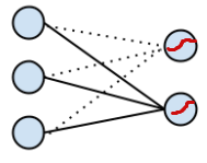
(注：虚线表示为 0 的权重，在第一张图中没有画出来，可以看到 logistic regression 就是 softmax regression 的一种特殊情况)

权重衰减 - 正则化

我们通过添加一个权重衰减项 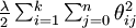 来修改代价函数（L2原理？），这个衰减项会惩罚过大的参数值，现在我们的代价函数变为：

有了这个权重衰减项以后 ()，代价函数就变成了严格的凸函数，这样就可以保证得到唯一的解了。 此时的 Hessian矩阵变为可逆矩阵，并且因为是凸函数，梯度下降法和 L-BFGS 等算法可以保证收敛到全局最优解。

为了使用优化算法，我们需要求得这个新函数  的导数，如下：

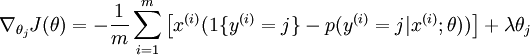
通过最小化 ，我们就能实现一个可用的 softmax 回归模型。

Softmax 回归 vs. k 个二元分类器

如果你在开发一个音乐分类的应用，需要对k种类型的音乐进行识别，那么是选择使用 softmax 分类器呢，还是使用 logistic 回归算法建立 k 个独立的二元分类器呢？

这一选择取决于你的类别之间是否互斥，

• • 例如，如果你有四个类别的音乐，分别为：古典音乐、乡村音乐、摇滚乐和爵士乐，那么你可以假设每个训练样本只会被打上一个标签（即：一首歌只能属于这四种音乐类型的其中一种），此时你应该使用类别数 k = 4 的softmax回归。（如果在你的数据集中，有的歌曲不属于以上四类的其中任何一类，那么你可以添加一个“其他类”，并将类别数 k 设为5。）
  • 如果你的四个类别如下：人声音乐、舞曲、影视原声、流行歌曲，那么这些类别之间并不是互斥的。例如：一首歌曲可以来源于影视原声，同时也包含人声 。这种情况下，使用4个二分类的 logistic 回归分类器更为合适。这样，对于每个新的音乐作品 ，我们的算法可以分别判断它是否属于各个类别。

现在我们来看一个计算视觉领域的例子，你的任务是将图像分到三个不同类别中。

• • (i) 假设这三个类别分别是：室内场景、户外城区场景、户外荒野场景。你会使用sofmax回归还是 3个logistic 回归分类器呢？ —— 三个类别是互斥的，因此更适于选择softmax回归分类器 。
  • (ii) 现在假设这三个类别分别是室内场景、黑白图片、包含人物的图片，你又会选择 softmax 回归还是多个 logistic 回归分类器呢？—— 建立三个独立的 logistic回归分类器更加合适。

 

例三： Plot multinomial and One-vs-Rest Logistic Regression

"""
====================================================
Plot multinomial and One-vs-Rest Logistic Regression
====================================================

Plot decision surface of multinomial and One-vs-Rest Logistic Regression.
The hyperplanes corresponding to the three One-vs-Rest (OVR) classifiers
are represented by the dashed lines.
"""
print(__doc__)
# Authors: Tom Dupre la Tour <tom.dupre-la-tour@m4x.org>
# License: BSD 3 clause

import numpy as np
import matplotlib.pyplot as plt
from sklearn.datasets import make_blobs
from sklearn.linear_model import LogisticRegression

# make 3-class dataset for classification
centers = [[-5, 0], [0, 1.5], [5, -1]]
X, y = make_blobs(n_samples=1000, centers=centers, random_state=40)
transformation = [[0.4, 0.2], [-0.4, 1.2]]
X = np.dot(X, transformation)

for multi_class in ('', 'ovr'):
    clf = LogisticRegression(solver='sag', max_iter=100, random_state=42, multi_class=multi_class).fit(X, y)

    # print the training scores
    print("training score : %.3f (%s)" % (clf.score(X, y), multi_class))

    # create a mesh to plot in
    h = .02  # step size in the mesh
    x_min, x_max = X[:, 0].min() - 1, X[:, 0].max() + 1
    y_min, y_max = X[:, 1].min() - 1, X[:, 1].max() + 1
    xx, yy = np.meshgrid(np.arange(x_min, x_max, h), np.arange(y_min, y_max, h))

    # Plot the decision boundary. For that, we will assign a color to each
    # point in the mesh [x_min, x_max]x[y_min, y_max].
    Z = clf.predict(np.c_[xx.ravel(), yy.ravel()])
    # Put the result into a color plot
    Z = Z.reshape(xx.shape)
    plt.figure()
    plt.contourf(xx, yy, Z, cmap=plt.cm.Paired)
    plt.title("Decision surface of LogisticRegression (%s)" % multi_class)
    plt.axis('tight')

    # Plot also the training points
    colors = "bry"
    for i, color in zip(clf.classes_, colors):
        idx = np.where(y == i)
        plt.scatter(X[idx, 0], X[idx, 1], c=color, cmap=plt.cm.Paired)

    # Plot the three one-against-all classifiers
    xmin, xmax = plt.xlim()
    ymin, ymax = plt.ylim()
    coef       = clf.coef_
    intercept  = clf.intercept_

    def plot_hyperplane(c, color):
        def line(x0):
            return (-(x0 * coef[c, 0]) - intercept[c]) / coef[c, 1]
        plt.plot([xmin, xmax], [line(xmin), line(xmax)],
                 ls="--", color=color)

    for i, color in zip(clf.classes_, colors):
        plot_hyperplane(i, color)

plt.show()

Result:

Jeff：可见multinomial是正确的选择。

End.