《DSP using MATLAB》 Problem 3.22

代码：

%% ------------------------------------------------------------------------
%%            Output Info about this m-file
fprintf('\n***********************************************************\n');
fprintf('        <DSP using MATLAB> Problem 3.22 \n\n');

banner();
%% ------------------------------------------------------------------------

%% -------------------------------------------------------------------
%%           1          xa(t)=cos(20πt+θ)  through A/D
%% -------------------------------------------------------------------
   Ts = 0.05;                        % sample interval, 0.05s
   Fs = 1/Ts;                        % Fs=20Hz
%theta = 0;
%theta = pi/6;
%theta = pi/4;
%theta = pi/3;
theta = pi/2;

n1_start = 0; n1_end = 20;
      n1 = [n1_start:1:n1_end];
     nTs = n1 * Ts;              % [0, 1]s

x1 = cos(20*pi*nTs + theta * ones(1,length(n1)));            % Digital signal

M = 500;
[X1, w] = dtft1(x1, n1, M);

magX1  = abs(X1);  angX1  = angle(X1);  realX1  = real(X1);  imagX1  = imag(X1);

%% --------------------------------------------------------------------
%%              START X(w)'s  mag ang real imag
%% --------------------------------------------------------------------
figure('NumberTitle', 'off', 'Name', sprintf('Problem 3.22 X1, theta/pi = %f', theta/pi));
set(gcf,'Color','white');
subplot(2,1,1); plot(w/pi,magX1); grid on;  %axis([-1,1,0,1.05]);
title('Magnitude Response');
xlabel('frequency in \pi units'); ylabel('Magnitude  |H|');
subplot(2,1,2); plot(w/pi, angX1/pi); grid on;  %axis([-1,1,-1.05,1.05]);
title('Phase Response');
xlabel('frequency in \pi units'); ylabel('Radians/\pi');

figure('NumberTitle', 'off', 'Name', sprintf('Problem 3.22 X1, theta/pi = %f', theta/pi));
set(gcf,'Color','white');
subplot(2,1,1); plot(w/pi, realX1); grid on;
title('Real Part');
xlabel('frequency in \pi units'); ylabel('Real');
subplot(2,1,2); plot(w/pi, imagX1); grid on;
title('Imaginary Part');
xlabel('frequency in \pi units'); ylabel('Imaginary');
%% -------------------------------------------------------------------
%%             END X's  mag ang real imag
%% -------------------------------------------------------------------

figure('NumberTitle', 'off', 'Name', sprintf('Problem 3.22 xa(n), theta/pi = %f and x1(n)', theta/pi));
na1 = 0:0.01:1;
xa1 = cos(20 * pi * na1 + theta * ones(1,length(na1)));
set(gcf, 'Color', 'white');
plot(1000*na1,xa1); grid on;  %axis([0,1,0,1.5]);
title('x1(n) and xa(n)');
xlabel('t in msec.'); ylabel('xa(t)'); hold on;
plot(1000*nTs, x1, 'o'); hold off;

%% ------------------------------------------------------------
%%                  xa(t) reconstruction from x1(n)
%% ------------------------------------------------------------

Dt = 0.001; t = 0:Dt:1;
xa = x1 * sinc(Fs*(ones(length(n1),1)*t - nTs'*ones(1,length(t)))) ;

figure('NumberTitle', 'off', 'Name', sprintf('Problem 3.22 Reconstructed From x1(n), theta/pi = %f', theta/pi));
set(gcf,'Color','white');
%subplot(2,1,1);
stairs(t*1000,xa,'r'); grid on;  %axis([0,1,0,1.5]);       % Zero-Order-Hold
title('Reconstructed Signal from x1(n) using Zero-Order-Hold');
xlabel('t in msec.'); ylabel('xa(t)'); hold on;
%stem(nTs*1000, x1); gtext('ZOH'); hold off;
plot(nTs*1000, x1, 'o'); gtext('ZOH'); hold off;

figure('NumberTitle', 'off', 'Name', sprintf('Problem 3.22 Reconstructed From x1(n), theta/pi = %f', theta/pi));
set(gcf,'Color','white');
%subplot(2,1,2);
plot(t*1000,xa,'r'); grid on;  %axis([0,1,0,1.5]);       % first-Order-Hold
title('Reconstructed Signal from x1(n) using First-Order-Hold');
xlabel('t in msec.'); ylabel('xa(t)'); hold on;
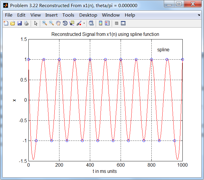
plot(nTs*1000,x1,'o'); gtext('FOH'); hold off;

xa = spline(nTs, x1, t);
figure('NumberTitle', 'off', 'Name', sprintf('Problem 3.22 Reconstructed From x1(n), theta/pi = %f', theta/pi));
set(gcf,'Color','white');
%subplot(2,1,1);
plot(1000*t, xa,'r');
xlabel('t in ms units'); ylabel('x');
title(sprintf('Reconstructed Signal from x1(n) using Spline function')); grid on; hold on;
plot(1000*nTs, x1,'o'); gtext('spline');

　　运行结果：

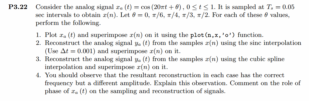
这里只看初相位为0的情况，原始模拟信号和采样信号（样点值圆圈标示）：

采样信号的谱，模拟角频率20π对应的数字角频率为π，如下图所示：

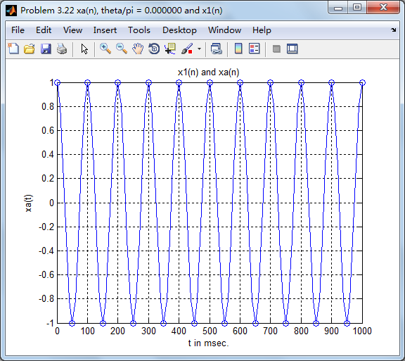
用采样信号重建原来模拟信号：

sinc方法，stairs函数画图

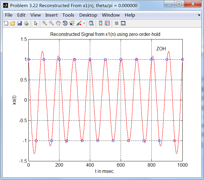
sinc方法，plot函数画图：

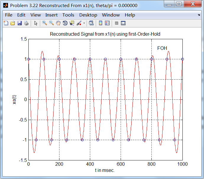
cubic方法

其他初相位的情况，这里不上图了。