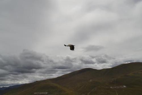
《DSP using MATLAB》Problem 8.22

时光飞逝，亲朋会一个一个离我们远去，孤独漂泊一阵子后，我们自己也要离开，

代码：

%% ------------------------------------------------------------------------
%%            Output Info about this m-file
fprintf('\n***********************************************************\n');
fprintf('        <DSP using MATLAB> Problem 8.22 \n\n');

banner();
%% ------------------------------------------------------------------------

% -------------------------------
%       ω = ΩT = 2πF/fs
% Digital Filter Specifications:
% -------------------------------
wp = 0.4*pi;                     % digital passband freq in rad/sec
ws = 0.6*pi;                     % digital stopband freq in rad/sec
Rp = 0.5;                        % passband ripple in dB
As = 50;                         % stopband attenuation in dB

Ripple = 10 ^ (-Rp/20)           % passband ripple in absolute
Attn = 10 ^ (-As/20)             % stopband attenuation in absolute

% Analog prototype specifications: Inverse Mapping for frequencies
T = 2;                       % set T = 1
Fs = 1/T;
OmegaP = wp/T;               % prototype passband freq
OmegaS = ws/T;               % prototype stopband freq

% Analog Butterworth Prototype Filter Calculation:
[cs, ds] = afd_butt(OmegaP, OmegaS, Rp, As);

% Calculation of second-order sections:
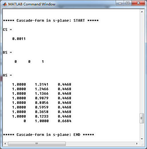
fprintf('\n***** Cascade-form in s-plane: START *****\n');
[CS, BS, AS] = sdir2cas(cs, ds)
fprintf('\n***** Cascade-form in s-plane: END *****\n');

% Calculation of Frequency Response:
[db_s, mag_s, pha_s, ww_s] = freqs_m(cs, ds, 0.5*pi);

% Calculation of Impulse Response:
[ha, x, t] = impulse(cs, ds);

% Impulse Invariance Transformation:
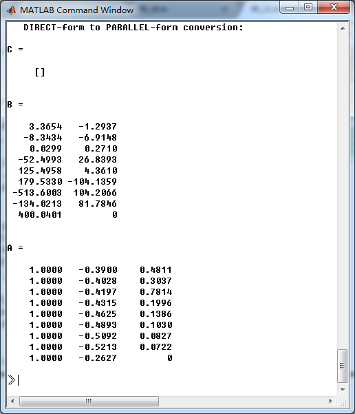
[b, a] = imp_invr(cs, ds, T); [C, B, A] = dir2par(b, a)

% Calculation of Frequency Response:
[db, mag, pha, grd, ww] = freqz_m(b, a);

%% -----------------------------------------------------------------
%%                             Plot
%% -----------------------------------------------------------------
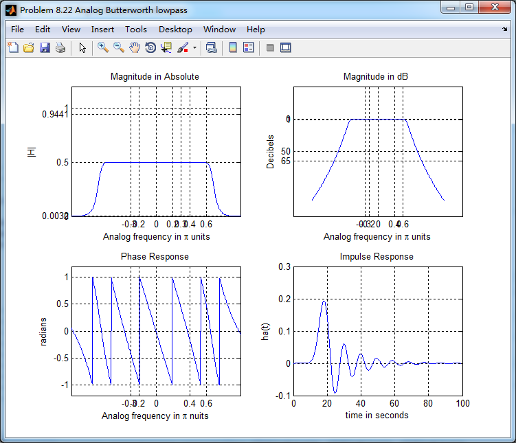
figure('NumberTitle', 'off', 'Name', 'Problem 8.22 Analog Butterworth lowpass')
set(gcf,'Color','white');
M = 1;                          % Omega max

subplot(2,2,1); plot(ww_s, mag_s/T);  grid on; axis([-M, M, 0, 1.2]);
xlabel(' Analog frequency in \pi units'); ylabel('|H|'); title('Magnitude in Absolute');
set(gca, 'XTickMode', 'manual', 'XTick', [-0.3, -0.2, 0, 0.2, 0.3, 0.4, 0.6]);
set(gca, 'YTickMode', 'manual', 'YTick', [0, 0.0032, 0.5, 0.9441, 1]);

subplot(2,2,2); plot(ww_s, db_s);  grid on; %axis([0, M, -50, 10]);
xlabel('Analog frequency in \pi units'); ylabel('Decibels'); title('Magnitude in dB ');
set(gca, 'XTickMode', 'manual', 'XTick', [-0.3, -0.2, 0, 0.4, 0.6]);
set(gca, 'YTickMode', 'manual', 'YTick', [-65, -50, -1, 0]);
set(gca,'YTickLabelMode','manual','YTickLabel',['65';'50';' 1';' 0']);

subplot(2,2,3); plot(ww_s, pha_s/pi);  grid on; axis([-M, M, -1.2, 1.2]);
xlabel('Analog frequency in \pi nuits'); ylabel('radians'); title('Phase Response');
set(gca, 'XTickMode', 'manual', 'XTick', [-0.3, -0.2, 0, 0.4, 0.6]);
set(gca, 'YTickMode', 'manual', 'YTick', [-1:0.5:1]);

subplot(2,2,4); plot(t, ha); grid on; %axis([0, 30, -0.05, 0.25]);
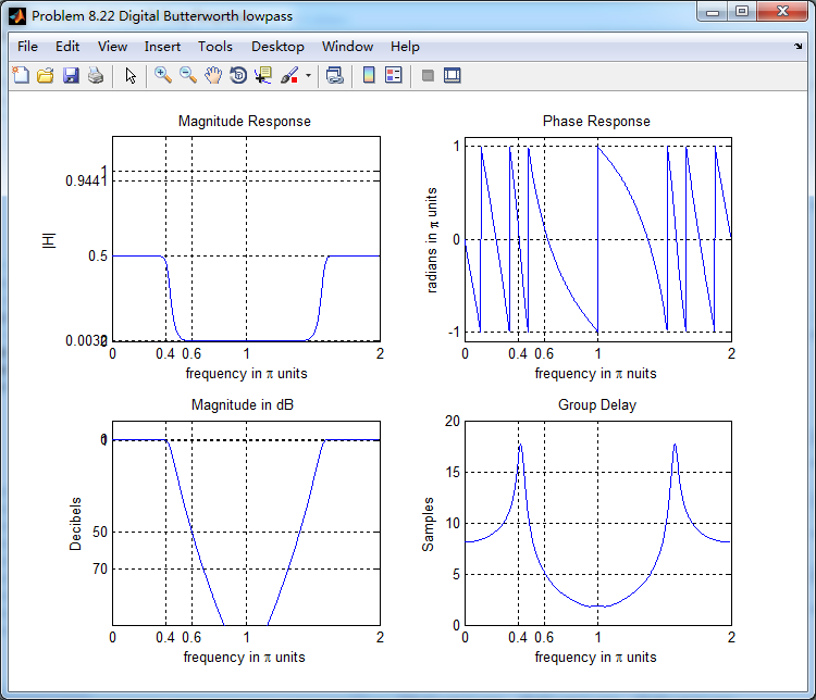
xlabel('time in seconds'); ylabel('ha(t)'); title('Impulse Response');

figure('NumberTitle', 'off', 'Name', 'Problem 8.22 Digital Butterworth lowpass')
set(gcf,'Color','white');
M = 2;                          % Omega max

subplot(2,2,1); plot(ww/pi, mag); axis([0, M, 0, 1.2]); grid on;
xlabel(' frequency in \pi units'); ylabel('|H|'); title('Magnitude Response');
set(gca, 'XTickMode', 'manual', 'XTick', [0, 0.4, 0.6, 1.0, M]);
set(gca, 'YTickMode', 'manual', 'YTick', [0, 0.0032, 0.5, 0.9441, 1]);

subplot(2,2,2); plot(ww/pi, pha/pi); axis([0, M, -1.1, 1.1]); grid on;
xlabel('frequency in \pi nuits'); ylabel('radians in \pi units'); title('Phase Response');
set(gca, 'XTickMode', 'manual', 'XTick', [0, 0.4, 0.6, 1.0, M]);
set(gca, 'YTickMode', 'manual', 'YTick', [-1:1:1]);

subplot(2,2,3); plot(ww/pi, db); axis([0, M, -100, 10]); grid on;
xlabel('frequency in \pi units'); ylabel('Decibels'); title('Magnitude in dB ');
set(gca, 'XTickMode', 'manual', 'XTick', [0, 0.4, 0.6, 1.0, M]);
set(gca, 'YTickMode', 'manual', 'YTick', [-70, -50, -1, 0]);
set(gca,'YTickLabelMode','manual','YTickLabel',['70';'50';' 1';' 0']);

subplot(2,2,4); plot(ww/pi, grd); grid on; %axis([0, M, 0, 35]);
xlabel('frequency in \pi units'); ylabel('Samples'); title('Group Delay');
set(gca, 'XTickMode', 'manual', 'XTick', [0, 0.4, 0.6, 1.0, M]);
%set(gca, 'YTickMode', 'manual', 'YTick', [0:5:35]);

figure('NumberTitle', 'off', 'Name', 'Problem 8.22 Pole-Zero Plot')
set(gcf,'Color','white');
zplane(b,a);
title(sprintf('Pole-Zero Plot'));
%pzplotz(b,a);

% ----------------------------------------------
%       Calculation of Impulse Response
% ----------------------------------------------
figure('NumberTitle', 'off', 'Name', 'Problem 8.22 Imp & Freq Response')
set(gcf,'Color','white');
t = [0:0.01:80]; subplot(2,1,1); impulse(cs,ds,t); grid on;   % Impulse response of the analog filter
axis([0,80,-0.2,0.3]);hold on

n = [0:1:80/T]; hn = filter(b,a,impseq(0,0,80/T));           % Impulse response of the digital filter
stem(n*T,hn); xlabel('time in sec'); title ('Impulse Responses');
hold off

% Calculation of Frequency Response:
[dbs, mags, phas, wws] = freqs_m(cs, ds, 2*pi/T);             % Analog frequency   s-domain  

[dbz, magz, phaz, grdz, wwz] = freqz_m(b, a);               % Digital  z-domain

%% -----------------------------------------------------------------
%%                             Plot
%% -----------------------------------------------------------------  

subplot(2,1,2); plot(wws/(2*pi),mags*Fs,'b+', wwz/(2*pi)*Fs,magz,'r'); grid on;

xlabel('frequency in Hz'); title('Magnitude Responses'); ylabel('Magnitude'); 

text(-0.3,0.15,'Analog filter'); text(0.4,0.55,'Digital filter');

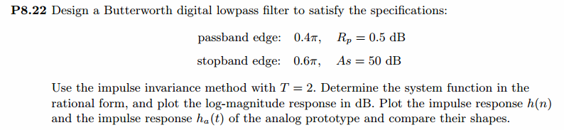
　　 运行结果：

通带、阻带绝对指标

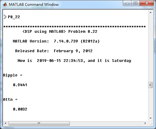
模拟原型butterworth低通滤波器直接形式系数

模拟原型butterworth低通滤波器串联形式系数

脉冲响应不变法，模拟低通转换成数字低通，并联形式系数