《DSP using MATLAB》Problem 7.31

参照Example7.27，因为0.1π=2πf1   f1=0.05，0.9π=2πf2   f2=0.45

所以0.1π≤ω≤0.9π，0.05≤|H|≤0.45

代码：

%% ++++++++++++++++++++++++++++++++++++++++++++++++++++++++++++++++++++++++++++++++
%%            Output Info about this m-file
fprintf('\n***********************************************************\n');
fprintf('        <DSP using MATLAB> Problem 7.31 \n\n');

banner();
%% ++++++++++++++++++++++++++++++++++++++++++++++++++++++++++++++++++++++++++++++++

f = [0  0.1  0.9   1];                          % in w/pi units
m = [0  0.05 0.45  0];                          % Magnitude values

M = 25;               % length of filter
N = M - 1;            % Nth-order
h = firpm(N, f, m, 'differentiator');
%h
[db, mag, pha, grd, w] = freqz_m(h, [1]);

[Hr, ww, c, L] = Hr_Type3(h);
%[Hr,omega,P,L] = ampl_res(h);

l = 0:M-1;
%% -------------------------------------------------
%%                    Plot
%% -------------------------------------------------
figure('NumberTitle', 'off', 'Name', 'Problem 7.31')
set(gcf,'Color','white');
subplot(2,2,1); plot(w/pi, db); grid on; axis([0 2 -90 10]);
set(gca,'YTickMode','manual','YTick',[-60,-40,-20,0])
set(gca,'YTickLabelMode','manual','YTickLabel',['60';'40';'20';' 0']);
set(gca,'XTickMode','manual','XTick',[0,0.1,0.9,1,1.1,1.9,2]);
xlabel('frequency in \pi units'); ylabel('Decibels'); title('Magnitude Response in dB');

subplot(2,2,3); plot(w/pi, mag); grid on; %axis([0 1 -100 10]);
xlabel('frequency in \pi units'); ylabel('Absolute'); title('Magnitude Response in absolute');
set(gca,'XTickMode','manual','XTick',[0,0.1,0.9,1,1.1,1.9,2]);
set(gca,'YTickMode','manual','YTick',[0,1.0,2.0]);

subplot(2,2,2); plot(w/pi, pha); grid on; %axis([0 1 -100 10]);
xlabel('frequency in \pi units'); ylabel('Rad'); title('Phase Response in Radians');
subplot(2,2,4); plot(w/pi, grd*pi/180);  grid on; %axis([0 1 -100 10]);
xlabel('frequency in \pi units'); ylabel('Rad'); title('Group Delay');

figure('NumberTitle', 'off', 'Name', 'Problem 7.31')
set(gcf,'Color','white'); 

subplot(2,2,1); stem(l, h); axis([-1, M, -0.6, 0.5]); grid on;
xlabel('n'); ylabel('h(n)'); title('Actual Impulse Response, M=25');
set(gca, 'XTickMode', 'manual', 'XTick', [0,12,25]);
set(gca, 'YTickMode', 'manual', 'YTick', [-0.6:0.2:0.6]);

subplot(2,2,3); plot(w/pi, db); axis([0, 1, -80, 10]); grid on;
xlabel('frequency in \pi units'); ylabel('Decibels'); title('Magnitude Response in dB ');
set(gca,'XTickMode','manual','XTick',f)
set(gca,'YTickMode','manual','YTick',[-60,-40,-20,0]);
set(gca,'YTickLabelMode','manual','YTickLabel',['60';'40';'20';' 0']);

subplot(2,2,4); plot(ww/pi, Hr); axis([0, 1, -0.2, 1.5]); grid on;
xlabel('frequency in \pi nuits'); ylabel('Hr(w)'); title('Amplitude Response');

n = [0:1:100];
x = 3*sin(0.25*pi*n);
y = filter(h,1,x);
y_chk = 0.75*cos(0.25*pi*n);

figure('NumberTitle', 'off', 'Name', 'Problem 7.31 x(n)')
set(gcf,'Color','white');
subplot(2,1,1); stem([0:M-1], h); axis([0 M-1 -0.5 0.5]); grid on;
xlabel('n'); ylabel('h(n)'); title('Actual Impulse Response, M=25');

subplot(2,1,2); stem(n, x); axis([0 100 0 3]); grid on;
xlabel('n'); ylabel('x(n)'); title('Input sequence');

figure('NumberTitle', 'off', 'Name', 'Problem 7.31 y(n) and y_chk(n)')
set(gcf,'Color','white');
subplot(2,1,1); stem(n, y); axis([0 100 -1 1]); grid on;
xlabel('n'); ylabel('y(n)'); title('Output sequence');

subplot(2,1,2); stem(n, y_chk); axis([0 100 -1 1]); grid on;
xlabel('n'); ylabel('y\_chk(n)'); title('Output sequence');

% ---------------------------
%    DTFT of x
% ---------------------------
MM = 500;
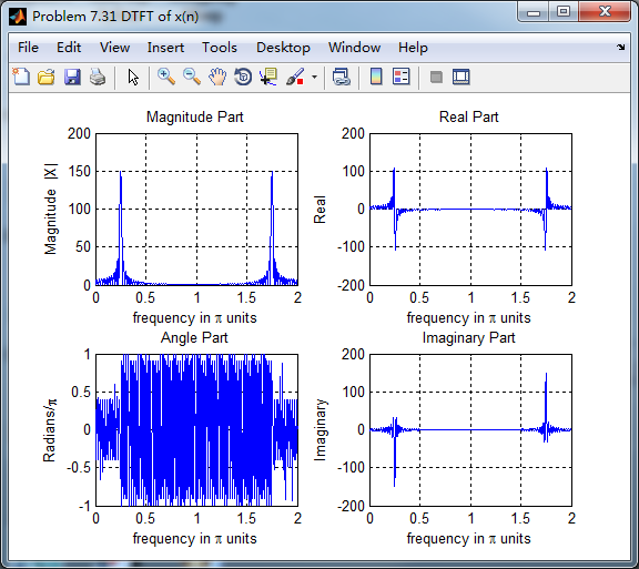
[X, w1] = dtft1(x, n, MM);
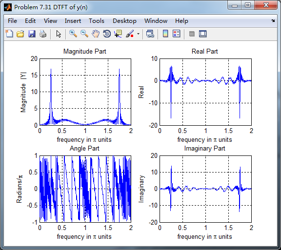
[Y, w1] = dtft1(y, n, MM);

magX = abs(X); angX = angle(X); realX = real(X); imagX = imag(X);
magY = abs(Y); angY = angle(Y); realY = real(Y); imagY = imag(Y);

figure('NumberTitle', 'off', 'Name', 'Problem 7.31 DTFT of x(n)')
set(gcf,'Color','white');
subplot(2,2,1); plot(w1/pi,magX); grid on; %axis([0,2,0,15]);
title('Magnitude Part');
xlabel('frequency in \pi units'); ylabel('Magnitude  |X|');
subplot(2,2,3); plot(w1/pi, angX/pi); grid on; axis([0,2,-1,1]);
title('Angle Part');
xlabel('frequency in \pi units'); ylabel('Radians/\pi');

subplot('2,2,2'); plot(w1/pi, realX); grid on;
title('Real Part');
xlabel('frequency in \pi units'); ylabel('Real');
subplot('2,2,4'); plot(w1/pi, imagX); grid on;
title('Imaginary Part');
xlabel('frequency in \pi units'); ylabel('Imaginary');

figure('NumberTitle', 'off', 'Name', 'Problem 7.31 DTFT of y(n)')
set(gcf,'Color','white');
subplot(2,2,1); plot(w1/pi,magY); grid on; %axis([0,2,0,15]);
title('Magnitude Part');
xlabel('frequency in \pi units'); ylabel('Magnitude  |Y|');
subplot(2,2,3); plot(w1/pi, angY/pi); grid on; axis([0,2,-1,1]);
title('Angle Part');
xlabel('frequency in \pi units'); ylabel('Radians/\pi');

subplot('2,2,2'); plot(w1/pi, realY); grid on;
title('Real Part');
xlabel('frequency in \pi units'); ylabel('Real');
subplot('2,2,4'); plot(w1/pi, imagY); grid on;
title('Imaginary Part');
xlabel('frequency in \pi units'); ylabel('Imaginary');

figure('NumberTitle', 'off', 'Name', 'Problem 7.31 Magnitude Response')
set(gcf,'Color','white');
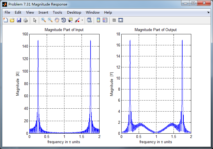
subplot(1,2,1); plot(w1/pi,magX); grid on; %axis([0,2,0,15]);
title('Magnitude Part of Input');
xlabel('frequency in \pi units'); ylabel('Magnitude  |X|');
subplot(1,2,2); plot(w1/pi,magY); grid on; %axis([0,2,0,15]);
title('Magnitude Part of Output');
xlabel('frequency in \pi units'); ylabel('Magnitude  |Y|');

　　运行结果：

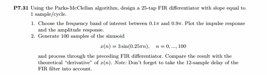
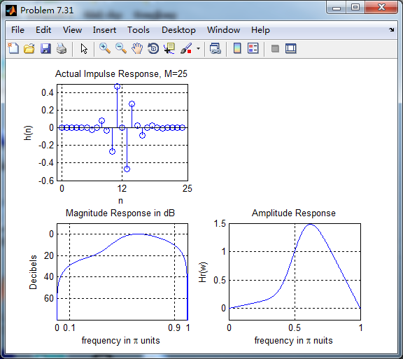
根据线性相位FIR性质，differentiator为第3类线性相位FIR，下图为脉冲响应、幅度谱和振幅谱。

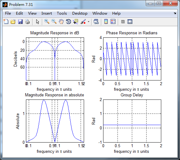
脉冲响应和输入序列

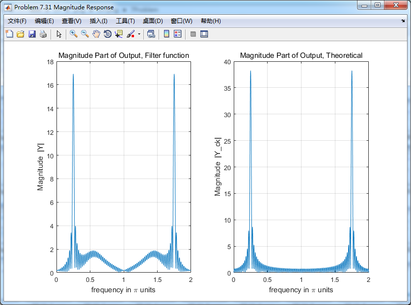
下图分别用卷积法和数学求导数方法得到的输出，

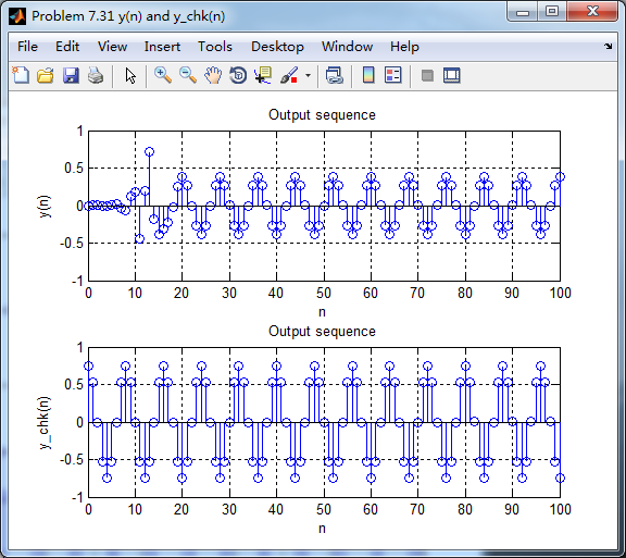
各自求其离散时间傅氏变换DTFT，得

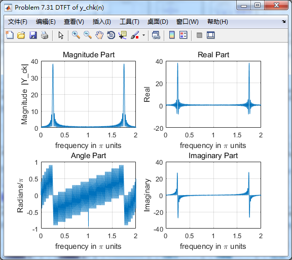
两种求微分结果幅度谱对比，可以看出：

1、设计滤波器卷积输入，输出的0.5π频率附近出现能量，数学求法没有；

2、设计滤波器卷积输入，幅度较数学求法小（能量有损失？）；