[Bayes] Understanding Bayes: Visualization of the Bayes Factor

From: https://alexanderetz.com/2015/08/09/understanding-bayes-visualization-of-bf/

Nearly被贝叶斯因子搞死，找篇神文舔。

---

In the first post of the Understanding Bayes series I said:

The likelihood is the workhorse of Bayesian inference.

In order to understand Bayesian parameter estimation you need to understand the likelihood. 参数估计 --> 似然

In order to understand Bayesian model comparison (Bayes factors) you need to understand the likelihood and likelihood ratios. 模型比较 --> 似然、似然比

I’ve shown in another post how the likelihood works as the updating factor for turning priors into posteriors for parameter estimation.

In this post I’ll explain how using Bayes factors for model comparison can be conceptualized as a simple extension of likelihood ratios.

如何使用贝叶斯因子比较模型。

There’s that coin again

Imagine we’re in a similar situation as before: I’ve flipped a coin 100 times and it came up 60 heads and 40 tails. The likelihood function for binomial data in general is:

and for this particular result:

The corresponding likelihood curve is shown below, which displays the relative likelihood for all possible simple (point) hypotheses given this data. Any likelihood ratio can be calculated by simply taking the ratio of the different hypotheses’s heights on the curve.

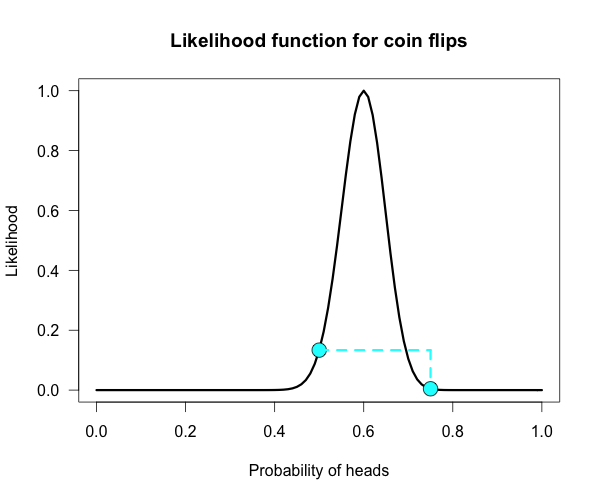
In that previous post I compared the fair coin hypothesis — H0: P(H)=.5 — vs one particular trick coin hypothesis — H1: P(H)=.75.

For 60 heads out of 100 tosses, the likelihood ratio for these hypotheses is L(.5)/L(.75) = 29.9. This means the data are 29.9 times as probable under the fair coin hypothesis than this particular trick coin hypothesis. 

But often we don’t have theories precise enough to make point predictions about parameters, at least not in psychology. So it’s often helpful if we can assign a range of plausible values for parameters as dictated by our theories.

传统俩模型的比较，采用这个似然函数比，感觉还不够好，还需要点更加正规的、有说服力的东西。

Enter the Bayes factor

Calculating a Bayes factor is a simple extension of this process. 贝叶斯因子 就是这么一个扩展。

A Bayes factor is a weighted average likelihood ratio, 有权重的、平均的、似然函数

where the weights are based on the prior distribution specified for the hypotheses. 权重基于先验。

For this example I’ll keep the simple fair coin hypothesis as the null hypothesis — H0: P(H)=.5 —

but now the alternative hypothesis will become a composite hypothesis — H1: P(θ).　　注意：未给定具体值，是一个变量。

(footnote 1) The likelihood ratio is evaluated at each point of P(θ) and weighted by the relative plausibility we assign that value.

Then once we’ve assigned weights to each ratio we just take the average to get the Bayes factor.

Figuring out how the weights should be assigned (the prior) is the tricky part.

Imagine my composite hypothesis, P(θ), is a combination of 21 different point hypotheses, all evenly spaced out between 0 and 1 and all of these points are weighted equally (not a very realistic hypothesis!).

So we end up with P(θ) = {0, .05, .10, .15, . . ., .9, .95, 1}. The likelihood ratio can be evaluated at every possible point hypothesis relative to H0,

and we need to decide how to assign weights. This is easy for this P(θ);

we assign zero weight for every likelihood ratio that is not associated with one of the point hypotheses contained in P(θ), and we assign weights of 1 to all likelihood ratios associated with the 21 points in P(θ).

21个点，代表不同的假设 in H1, 不同的点 对应 不同的 似然值。

This gif has the 21 point hypotheses of P(θ) represented as blue vertical lines (indicating where we put our weights of 1), and

the turquoise tracking lines represent the likelihood ratio being calculated at every possible point relative to H0: P(H)=.5.

(Remember, the likelihood ratio is the ratio of the heights on the curve.)

This means we only care about the ratios given by the tracking lines when the dot attached to the moving arm aligns with the vertical P(θ) lines. [edit: this paragraph added as clarification]

The 21 likelihood ratios associated with P(θ) are:

{~0, ~0, ~0, ~0, ~0, ~0, ~0, ~0, .002, .08, 1, 4.5, 7.5, 4.4, .78, .03, ~0, ~0, ~0, ~0, ~0}

Since they are all weighted equally we simply average, and obtain BF = 18.3/21 = .87. 所有似然值的均值，暂时用离散的方式。

In other words, the data (60 heads out of 100) are 1/.87 = 1.15 times more probable under the null hypothesis — H0: P(H)=.5 — than this particular composite hypothesis — H1: P(θ). 这也可以认为是组合假设

Entirely uninformative!

Despite tossing the coin 100 times we have extremely weak evidence that is hardly worth even acknowledging.

This happened because much of P(θ) falls in areas of extremely low likelihood relative to H0, as evidenced by those 13 zeros above.

P(θ) is flexible, since it covers the entire possible range of θ, but this flexibility comes at a price. You have to pay for all of those zeros with a lower weighted average and a smaller Bayes factor.

可见，有太多的可能性导致的似然过于低，这便造成了一些影响：虽然0.6（from data）看似更好，但0.5的H0假设实际算来，其实更合理。完全没信息的先验反而胜利了！

下面，忽略掉这些似然值低的点，看看会发生什么。

Now imagine I had seen a trick coin like this before, and I know it had a slight bias towards landing heads. 假设头的概率高些。

I can use this information to make more pointed predictions. Let’s say I define P(θ) as 21 equally weighted point hypotheses again,

but this time they are all equally spaced between .5 and .75,

which happens to be the highest density region of the likelihood curve (how fortuitous!). Now P(θ) = {.50, .5125, .525, . . ., .7375, .75}. 还是21份.

The 21 likelihood ratios associated with the new P(θ) are:

{1.00, 1.5, 2.1, 2.8, 4.5, 5.4, 6.2, 6.9, 7.5, 7.3, 6.9, 6.2, 4.4, 3.4, 2.6, 1.8, .78, .47, .27, .14, .03}

They are all still weighted equally, so the simple average is BF = /21 = 3.4.

Three times more informative than before, and in favor of P(θ) this time! 这次又不再倾向于无信息先验咯！

And no zeros. We were able to add theoretically relevant information to H1 to make more accurate predictions, and we get rewarded with a Bayes boost. (But this result is only 3-to-1 evidence, which is still fairly weak.)

This new P(θ) is risky though, because if the data show a bias towards tails or a more extreme bias towards heads then it faces a very heavy penalty (many more zeros).

实际代表：先验与实际的样本有较大的不吻合，该怎么办？

High risk = high reward with the Bayes factor.

Make pointed predictions that match the data and get a bump to your BF, but if you’re wrong then pay a steep price.

For example, if the data were 60 tails instead of 60 heads the BF would be 10-to-1 against P(θ) rather than 3-to-1 for P(θ)!

Now, typically people don’t actually specify hypotheses like these. Typically they use continuous distributions, but the idea is the same.

再扩展到连续的情况。

Take the likelihood ratio at each point relative to H0, weigh according to plausibilities given in P(θ), and then average.

A more realistic (?) example

Imagine you’re walking down the sidewalk and you see a shiny piece of foreign currency by your feet. You pick it up and want to know if it’s a fair coin or an unfair coin. As a Bayesian you have to be precise about what you mean by fair and unfair.

Fair is typically pretty straightforward — H0: P(H)=.5 as before — but unfair could mean anything. （H1假设 是个范围）

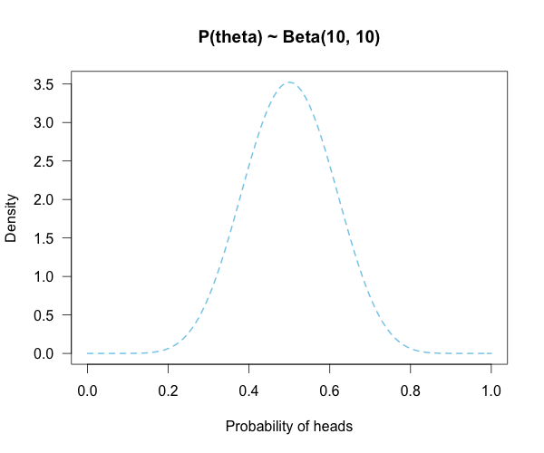
Since this is a completely foreign coin to you, you may want to be fairly open-minded about it. After careful deliberation, you assign P(θ) a beta distribution, with shape parameters 10 and 10. （H1假设了一个分布）

That is, H1: P(θ) ~ Beta(10, 10).

This means that if the coin isn’t fair, it’s probably close to fair but it could reasonably be moderately biased, and you have no reason to think it is particularly biased to one side or the other.

是的，起初，一个未知的硬币，怎么可能臆想bias的细节呢？我们需要实验数据。

Now you build a perfect coin-tosser machine and set it to toss 100 times (but not any more than that because you haven’t got all day). You carefully record the results and the coin comes up 33 heads out of 100 tosses.

实验数据：33个头，似然值目前最佳是：33/100，即：似然的curve是确定的。

H0：一个值，即 0.5

H1：一个分布，包含很多值，每个值还有概率（权重）

Under which hypothesis are these data more probable, H0 or H1? In other words, which hypothesis did the better job predicting these data?

This may be a continuous prior but the concept is exactly the same as before: weigh the various likelihood ratios based on the prior plausibility assignment and then average.

The continuous distribution on P(θ) can be thought of as a set of many many point hypotheses spaced very very close together.

So if the range of θ we are interested in is limited to 0 to 1, as with binomials and coin flips,

then a distribution containing 101 point hypotheses spaced .01 apart, can effectively be treated as if it were continuous.

The numbers will be a little off but all in all it’s usually pretty close. So imagine that instead of 21 hypotheses you have 101, and their relative plausibilities follow the shape of a Beta(10, 10). (footnote 2)

Since this is not a uniform distribution, we need to assign varying weights to each likelihood ratio.

对于H0：一个值，即 0.5，计算似然值即可。

对于H1：一个分布，包含很多值，每个值还有概率（权重），需要综合考虑，计算一个期望值。

Each likelihood ratio associated with a point in P(θ) is simply multiplied by the respective density assigned to it under P(θ).

For example, the density of P(θ) at .4 is 2.44. So we multiply the likelihood ratio at that point, L(.4)/L(.5) = 128, by 2.44, and add it to the accumulating total likelihood ratio.

Do this for every point and then divide by the total number of points, in this case 101, to obtain the approximate Bayes factor. The total weighted likelihood ratio is 5564.9, divide it by 101 to get 55.1, and there’s the Bayes factor. In other words, the data are roughly 55 times more probable under this composite H1 than under H0. The alternative hypothesis H1 did a much better job predicting these data than did the null hypothesis H0.

The actual Bayes factor is obtained by integrating the likelihood with respect to H1’s density distribution and then dividing by the (marginal) likelihood of H0.

Essentially what it does is cut P(θ) into slices infinitely thin before it calculates the likelihood ratios, re-weighs, and averages. That Bayes factor comes out to 55.7, which is basically the same thing we got through this ghetto visualization demonstration!

Take home

The take-home message is hopefully pretty clear at this point: When you are comparing a point null hypothesis with a composite hypothesis,

the Bayes factor can be thought of as a weighted average of every point hypothesis’s likelihood ratio against H0, and

the weights are determined by the prior density distribution of H1.

Since the Bayes factor is a weighted average based on the prior distribution, it’s really important to think hard about the prior distribution you choose for H1.

因为这个原因，所以先验的选择才需要重视。

In a previous post, I showed how different priors can converge to the same posterior with enough data. The priors are often said to “wash out” in estimation problems like that. This is not necessarily the case for Bayes factors. The priors you choose matter, so think hard!

## Plots the likelihood function for the data obtained
## h = number of successes (heads), n = number of trials (flips),
## p1 = prob of success (head) on H1, p2 = prob of success (head) on H0
#the auto plot loop is taken from http://www.r-bloggers.com/automatically-save-your-plots-to-a-folder/
#and then the pngs are combined into a gif online 

LR <- function(h,n,p1=seq(0,1,.01),p2=rep(.5,101)){
  L1 <- dbinom(h,n,p1)/dbinom(h,n,h/n) ## Likelihood for p1, standardized vs the MLE
  L2 <- dbinom(h,n,p2)/dbinom(h,n,h/n) ## Likelihood for p2, standardized vs the MLE
  Ratio <<- dbinom(h,n,p1)/dbinom(h,n,p2) ## Likelihood ratio for p1 vs p2, saves to global workspace with <<-
  x<- seq(0,1,.01) #sets up for loop
  m<- seq(0,1,.01) #sets up for p(theta)
  ym<-dbeta(m,10,10) #p(theta) densities
  names<-seq(1,length(x),1) #names for png loop
  for(i in 1:length(x)){
    mypath<-file.path("~",paste("myplot_", names[i], ".png", sep = "")) #set up for save file path
    png(file=mypath, width=1200,height=1000,res=200) #the next plotted item saves as this png format
    curve(3.5*(dbinom(h,n,x)/max(dbinom(h,n,h/n))), ylim=c(0,3.5), xlim = c(0,1), ylab = "Likelihood",
          xlab = "Probability of heads",las=1, main = "Likelihood function for coin flips", lwd = 3)

    lines(m,ym, type="h", lwd=1, lty=2, col="skyblue" ) #p(theta) density

    points(p1[i], 3.5*L1[i], cex = 2, pch = 21, bg = "cyan") #tracking dot
    points(p2, 3.5*L2, cex = 2, pch = 21, bg = "cyan") #stationary null dot
    #abline(v = h/n, lty = 5, lwd = 1, col = "grey73") #un-hash if you want to add a line at the MLE

    lines(c(p1[i], p1[i]), c(3.5*L1[i], 3.6), lwd = 3, lty = 2, col = "cyan") #adds vertical line at p1
    lines(c(p2[i], p2[i]), c(3.5*L2[i], 3.6), lwd = 3, lty = 2, col = "cyan") #adds vertical line at p2, fixed at null
    lines(c(p1[i], p2[i]), c(3.6, 3.6), lwd=3,lty=2,col="cyan") #adds horizontal line connecting them
    dev.off() #lets you save directly

  }

}

LR(33,100) #executes the final example
v<-seq(0,1,.05) #the segments of P(theta) when it is uniform
sum(Ratio[v]) #total weighted likelihood ratio
mean(Ratio[v]) #average weighted likelihood ratio (i.e., BF)

x<- seq(0,1,.01) #segments for p(theta)~beta
y<-dbeta(x,10,10) #assigns densitys for P(theta)
k=sum(y*Ratio) #multiply likelihood ratios by the density under P(theta)
l=k/101 #weighted average likelihood ratio (i.e., BF)

小心，程序会生成动画101帧的图片。：）