Logistic回归 python实现

Logistic回归

算法优缺点：

1.计算代价不高，易于理解和实现
2.容易欠拟合，分类精度可能不高
3.适用数据类型：数值型和标称型

算法思想：

• 其实就我的理解来说，logistic回归实际上就是加了个sigmoid函数的线性回归，这个sigmoid函数的好处就在于，将结果归到了0到1这个区间里面了，并且sigmoid（0）=0.5，也就是说里面的线性部分的结果大于零小于零就可以直接计算到了。这里的求解方式是梯度上升法，具体我就不扯了，最推荐的资料还是Ng的视频，那里面的梯度下降就是啦，只不过一个是梯度上升的方向一个是下降的方向，做法什么的都一样。
• 而梯度上升（准确的说叫做“批梯度上升”）的一个缺点就是计算量太大了，每一次迭代都需要把所有的数据算一遍，这样一旦训练集大了之后，那么计算量将非常大，所以这里后面还提出了随机梯度下降，思想就是每次只是根据一个data进行修正。这样得到的最终的结果可能会有所偏差但是速度却提高了很多，而且优化之后的偏差还是很小的。随机梯度上升的另一个好处是这是一个在线算法，可以根据新数据的到来不断处理

函数：

loadDataSet()
创建数据集，这里的数据集就是在一个文件中，这里面有三行，分别是两个特征和一个标签，但是我们在读出的时候还加了X0这个属性
sigmoid(inX)
sigmoid函数的计算，这个函数长这样的，基本坐标大点就和阶跃函数很像了

gradAscend(dataMatIn, classLabels)
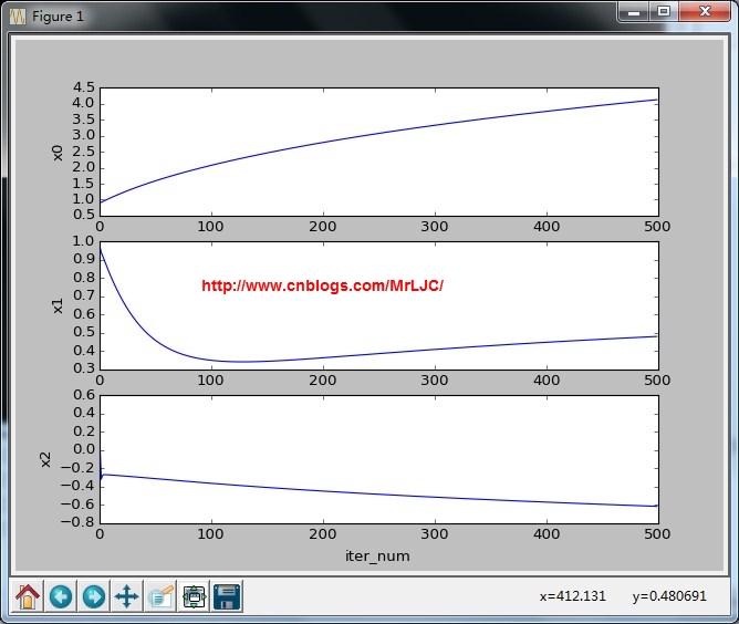
梯度上升算法的实现，里面用到了numpy的数组，并且设定了迭代次数500次，然后为了计算速度都采取了矩阵计算，计算的过程中的公式大概是：w= w+alpha*(y-h)x[i]（一直懒得写公式，见谅。。。）
gradAscendWithDraw(dataMatIn, classLabels)
上面的函数加强版，增加了一个weight跟着迭代次数的变化曲线
stocGradAscent0(dataMatrix, classLabels)
这里为了加快速度用来随机梯度上升，即每次根据一组数据调整（额，好吧，这个际没有随机因为那是线面那个函数）
stocGradAscentWithDraw0(dataMatrix, classLabels)
上面的函数加强版，增加了一个weight跟着迭代次数的变化曲线
stocGradAscent1(dataMatrix, classLabels, numIter=150)
这就真的开始随机了，随机的主要好处是减少了周期性的波动了。另外这里还加入了alpha的值随迭代变化，这样可以让alpha的值不断的变化，但是都不会减小到0。
stocGradAscentWithDraw1(dataMatrix, classLabels, numIter=150)
上面的函数加强版，增加了一个weight跟着迭代次数的变化曲线
plotBestFit(wei)
根据计算的weight值画出拟合的线，直观观察效果

运行效果分析：

1、梯度上升：

迭代变化趋势

分类结果：

2、随机梯度上升版本1

迭代变化趋势

分类结果：

这个速度虽然快了很多但是效果不太理想啊。不过这个计算量那么少，我们如果把这个迭代200次肯定不一样了，效果如下

果然好多了

3、随机梯度上升版本2

迭代变化趋势

分类结果：

恩，就是这样啦，效果还是不错的啦。代码的画图部分写的有点烂，见谅啦

1.  #coding=utf-8
    from numpy import *
   
    def loadDataSet():
        dataMat = []
        labelMat = []
        fr = open('testSet.txt')
        for line in fr.readlines():
            lineArr = line.strip().split()
            dataMat.append([1.0, float(lineArr[0]), float(lineArr[1])])
            labelMat.append(int(lineArr[2]))
        return dataMat, labelMat
   
    def sigmoid(inX):
        return 1.0/(1+exp(-inX))
   
    def gradAscend(dataMatIn, classLabels):
        dataMatrix = mat(dataMatIn)
        labelMat = mat(classLabels).transpose()
        m,n = shape(dataMatrix)
        alpha = 0.001
        maxCycle = 500
        weight = ones((n,1))
        for k in range(maxCycle):
            h = sigmoid(dataMatrix*weight)
            error = labelMat - h
            weight += alpha * dataMatrix.transpose() * error
            #plotBestFit(weight)
        return weight
   
    def gradAscendWithDraw(dataMatIn, classLabels):
        import matplotlib.pyplot as plt
        fig = plt.figure()
        ax = fig.add_subplot(311,ylabel='x0')
        bx = fig.add_subplot(312,ylabel='x1')
        cx = fig.add_subplot(313,ylabel='x2')
        dataMatrix = mat(dataMatIn)
        labelMat = mat(classLabels).transpose()
        m,n = shape(dataMatrix)
        alpha = 0.001
        maxCycle = 500
        weight = ones((n,1))
        wei1 = []
        wei2 = []
        wei3 = []
        for k in range(maxCycle):
            h = sigmoid(dataMatrix*weight)
            error = labelMat - h
            weight += alpha * dataMatrix.transpose() * error
            wei1.extend(weight[0])
            wei2.extend(weight[1])
            wei3.extend(weight[2])
        ax.plot(range(maxCycle), wei1)
        bx.plot(range(maxCycle), wei2)
        cx.plot(range(maxCycle), wei3)
        plt.xlabel('iter_num')
        plt.show()
        return weight
   
    def stocGradAscent0(dataMatrix, classLabels):
        m,n = shape(dataMatrix)
   
        alpha = 0.001
        weight = ones(n)
        for i in range(m):
            h = sigmoid(sum(dataMatrix[i]*weight))
            error = classLabels[i] - h
            weight = weight + alpha * error * dataMatrix[i]
        return weight
   
    def stocGradAscentWithDraw0(dataMatrix, classLabels):
        import matplotlib.pyplot as plt
        fig = plt.figure()
        ax = fig.add_subplot(311,ylabel='x0')
        bx = fig.add_subplot(312,ylabel='x1')
        cx = fig.add_subplot(313,ylabel='x2')
        m,n = shape(dataMatrix)
   
        alpha = 0.001
        weight = ones(n)
        wei1 = array([])
        wei2 = array([])
        wei3 = array([])
        numIter = 200
        for j in range(numIter):
            for i in range(m):
                h = sigmoid(sum(dataMatrix[i]*weight))
                error = classLabels[i] - h
                weight = weight + alpha * error * dataMatrix[i]
                wei1 =append(wei1, weight[0])
                wei2 =append(wei2, weight[1])
                wei3 =append(wei3, weight[2])
        ax.plot(array(range(m*numIter)), wei1)
        bx.plot(array(range(m*numIter)), wei2)
        cx.plot(array(range(m*numIter)), wei3)
        plt.xlabel('iter_num')
        plt.show()
        return weight
   
    def stocGradAscent1(dataMatrix, classLabels, numIter=150):
        m,n = shape(dataMatrix)
   
        #alpha = 0.001
        weight = ones(n)
        for j in range(numIter):
            dataIndex = range(m)
            for i in range(m):
                alpha = 4/ (1.0+j+i) +0.01
                randIndex = int(random.uniform(0,len(dataIndex)))
                h = sigmoid(sum(dataMatrix[randIndex]*weight))
                error = classLabels[randIndex] - h
                weight = weight + alpha * error * dataMatrix[randIndex]
                del(dataIndex[randIndex])
        return weight
   
    def stocGradAscentWithDraw1(dataMatrix, classLabels, numIter=150):
        import matplotlib.pyplot as plt
        fig = plt.figure()
        ax = fig.add_subplot(311,ylabel='x0')
        bx = fig.add_subplot(312,ylabel='x1')
        cx = fig.add_subplot(313,ylabel='x2')
        m,n = shape(dataMatrix)
   
        #alpha = 0.001
        weight = ones(n)
        wei1 = array([])
        wei2 = array([])
        wei3 = array([])
        for j in range(numIter):
            dataIndex = range(m)
            for i in range(m):
                alpha = 4/ (1.0+j+i) +0.01
                randIndex = int(random.uniform(0,len(dataIndex)))
                h = sigmoid(sum(dataMatrix[randIndex]*weight))
                error = classLabels[randIndex] - h
                weight = weight + alpha * error * dataMatrix[randIndex]
                del(dataIndex[randIndex])
                wei1 =append(wei1, weight[0])
                wei2 =append(wei2, weight[1])
                wei3 =append(wei3, weight[2])
        ax.plot(array(range(len(wei1))), wei1)
        bx.plot(array(range(len(wei2))), wei2)
        cx.plot(array(range(len(wei2))), wei3)
        plt.xlabel('iter_num')
        plt.show()
        return weight
   
    def plotBestFit(wei):
        import matplotlib.pyplot as plt
        weight = wei
        dataMat,labelMat = loadDataSet()
        dataArr = array(dataMat)
        n = shape(dataArr)[0]
        xcord1 = []
        ycord1 = []
        xcord2 = []
        ycord2 = []
        for i in range(n):
            if int(labelMat[i]) == 1:
                xcord1.append(dataArr[i,1])
                ycord1.append(dataArr[i,2])
            else:
                xcord2.append(dataArr[i,1])
                ycord2.append(dataArr[i,2])
        fig = plt.figure()
        ax = fig.add_subplot(111)
        ax.scatter(xcord1, ycord1, s=30, c='red', marker='s')
        ax.scatter(xcord2, ycord2, s=30, c='green')
        x = arange(-3.0, 3.0, 0.1)
        y = (-weight[0] - weight[1]*x)/weight[2]
        ax.plot(x,y)
        plt.xlabel('X1')
        plt.ylabel('X2')
        plt.show()
   
    def main():
        dataArr,labelMat = loadDataSet()
        #w = gradAscendWithDraw(dataArr,labelMat)
        w = stocGradAscentWithDraw0(array(dataArr),labelMat)
        plotBestFit(w)
   
    if __name__ == '__main__':
        main()

   机器学习笔记索引

来自为知笔记(Wiz)