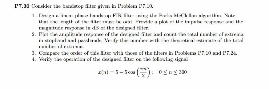
《DSP using MATLAB》Problem 7.30

代码：

%% ++++++++++++++++++++++++++++++++++++++++++++++++++++++++++++++++++++++++++++++++
%%            Output Info about this m-file
fprintf('\n***********************************************************\n');
fprintf('        <DSP using MATLAB> Problem 7.30 \n\n');

banner();
%% ++++++++++++++++++++++++++++++++++++++++++++++++++++++++++++++++++++++++++++++++

% bandstop, Length MUST be odd number.
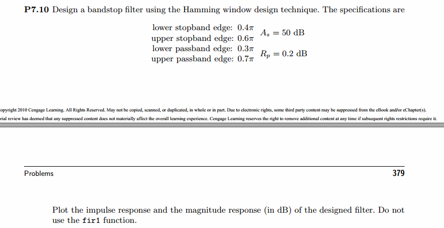
wp1 = 0.3*pi; ws1 = 0.4*pi; ws2 = 0.6*pi; wp2 = 0.7*pi;
As = 50; Rp = 0.2;

[delta1, delta2] = db2delta(Rp, As);
deltaH = max(delta1,delta2); deltaL = min(delta1,delta2);

f = [wp1, ws1, ws2, wp2]/pi; m = [1, 0, 1]; delta = [delta1, delta2, delta1];

[N, f, m, weights] = firpmord(f, m, delta);
N

h = firpm(N, f, m, weights);
[db, mag, pha, grd, w] = freqz_m(h, [1]);
delta_w = 2*pi/1000;
wp1i = floor(wp1/delta_w)+1; ws1i = floor(ws1/delta_w)+1;
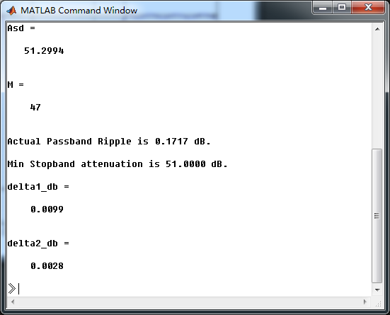
ws2i = floor(ws2/delta_w)+1; wp2i = floor(wp2/delta_w)+1;

Asd = -max(db(ws1i : 1 : ws2i))

M = N + 1
l = 0:M-1;
%% --------------------------------------------------
%%                   Type-1 BPF
%% --------------------------------------------------
[Hr, ww, a, L] = Hr_Type1(h);

Rp = -(min(db(1:1: wp1i)));                   % Actual Passband Ripple
fprintf('\nActual Passband Ripple is %.4f dB.\n', Rp);

As = -round(max(db(ws1i : 1 : ws2i)));        % Min Stopband attenuation
fprintf('\nMin Stopband attenuation is %.4f dB.\n', As);

[delta1_db, delta2_db] = db2delta(Rp, As)

% Plot
figure('NumberTitle', 'off', 'Name', 'Problem 7.30 h(n), Parks-McClellan Method')
set(gcf,'Color','white');
subplot(2,2,1); stem([0:M-1], h); axis([0 M-1 -0.3 0.7]); grid on;
xlabel('n'); ylabel('h(n)'); title('Actual Impulse Response, M=47');

subplot(2,2,2); plot(w/pi, db); axis([0 1 -90 10]); grid on;
set(gca,'YTickMode','manual','YTick',[-51,-9,0])
set(gca,'YTickLabelMode','manual','YTickLabel',['51';' 9';' 0']);
set(gca,'XTickMode','manual','XTick',[0,0.3,0.4,0.6,0.7,1]);
xlabel('frequency in \pi units'); ylabel('Decibels'); title('Magnitude Response in dB');

subplot(2,2,3); plot(ww/pi, Hr); axis([0, 1, -0.2, 1.2]); grid on;
xlabel('frequency in \pi nuits'); ylabel('Hr(w)'); title('Amplitude Response');
set(gca,'XTickMode','manual','XTick',[0,0.3,0.4,0.6,0.7,1])
set(gca,'YTickMode','manual','YTick',[0,1]);

subplot(2,2,4);
pb1w = ww(1:1:wp1i)/pi; pb1e = Hr(1:1:wp1i)-1;
sbw = ww(ws1i:ws2i)/pi; sbe = Hr(ws1i:ws2i);
pb2w = ww(wp2i:501)/pi; pb2e = Hr(wp2i:501)-1;
plot(pb1w,pb1e*(delta2/delta1), sbw,sbe, pb2w,pb2e*(delta2/delta1));   % weighted error
% plot(pb1w,pb1e, sbw,sbe, pb2w,pb2e);  % error

axis([0, 1, -deltaL, deltaL]); grid on;
xlabel('frequency in \pi units'); ylabel('Hr(w)');
title('Weighted Error');
%title('Error Response');
set(gca,'XTickMode','manual','XTick',f)
set(gca,'YTickMode','manual','YTick',[-deltaL, 0,deltaL]);
set(gca,'XGrid','on','YGrid','on')

figure('NumberTitle', 'off', 'Name', 'Problem 7.30 Parks-McClellan Method')
set(gcf,'Color','white');
subplot(2,2,1); plot(w/pi, db); grid on; axis([0 2 -90 10]);
set(gca,'YTickMode','manual','YTick',[-51,-9,0])
set(gca,'YTickLabelMode','manual','YTickLabel',['51';' 9';' 0']);
set(gca,'XTickMode','manual','XTick',[0,0.3,0.4,0.6,0.7,1,1.3,1.4,1.6,1.7,2]);
xlabel('frequency in \pi units'); ylabel('Decibels'); title('Magnitude Response in dB');

subplot(2,2,3); plot(w/pi, mag); grid on; %axis([0 1 -100 10]);
xlabel('frequency in \pi units'); ylabel('Absolute'); title('Magnitude Response in absolute');
set(gca,'XTickMode','manual','XTick',[0,0.3,0.4,0.6,0.7,1,1.3,1.4,1.6,1.7,2]);
set(gca,'YTickMode','manual','YTick',[0,1.0]);

subplot(2,2,2); plot(w/pi, pha); grid on; %axis([0 1 -100 10]);
xlabel('frequency in \pi units'); ylabel('Rad'); title('Phase Response in Radians');
subplot(2,2,4); plot(w/pi, grd*pi/180);  grid on; %axis([0 1 -100 10]);
xlabel('frequency in \pi units'); ylabel('Rad'); title('Group Delay');

figure('NumberTitle', 'off', 'Name', 'Problem 7.30 AmpRes of h(n), Parks-McClellan Method')
set(gcf,'Color','white'); 

plot(ww/pi, Hr); grid on; %axis([0 1 -100 10]);
xlabel('frequency in \pi units'); ylabel('Hr'); title('Amplitude Response');
set(gca,'YTickMode','manual','YTick',[-delta2_db ,0,delta2_db , 1-delta1_db, 1, 1+delta1_db]);
set(gca,'XTickMode','manual','XTick',[0,0.3,0.4,0.6,0.7,1]);

n = [0:1:300];
x = 5-5*cos(pi*n/2);
y = filter(h,1,x);

figure('NumberTitle', 'off', 'Name', 'Problem 7.30 x(n) and y(n)')
set(gcf,'Color','white');
subplot(3,1,1); stem([0:M-1], h); axis([0 M-1 -0.3 0.7]); grid on;
xlabel('n'); ylabel('h(n)'); title('Actual Impulse Response, M=47');

subplot(3,1,2); stem(n, x); axis([0 300 0 10]); grid on;
xlabel('n'); ylabel('x(n)'); title('Input sequence');

subplot(3,1,3); stem(n, y); axis([0 100 -5 7]); grid on;
xlabel('n'); ylabel('y(n)'); title('Output sequence');

% ---------------------------
%    DTFT of x
% ---------------------------
MM = 500;
[X, w1] = dtft1(x, n, MM);
[Y, w1] = dtft1(y, n, MM);

magX = abs(X); angX = angle(X); realX = real(X); imagX = imag(X);
magY = abs(Y); angY = angle(Y); realY = real(Y); imagY = imag(Y);

figure('NumberTitle', 'off', 'Name', 'Problem 7.30 DTFT of x(n)')
set(gcf,'Color','white');
subplot(2,2,1); plot(w1/pi,magX); grid on; %axis([0,2,0,15]);
title('Magnitude Part');
xlabel('frequency in \pi units'); ylabel('Magnitude  |X|');
subplot(2,2,3); plot(w1/pi, angX/pi); grid on; axis([0,2,-1,1]);
title('Angle Part');
xlabel('frequency in \pi units'); ylabel('Radians/\pi');

subplot('2,2,2'); plot(w1/pi, realX); grid on;
title('Real Part');
xlabel('frequency in \pi units'); ylabel('Real');
subplot('2,2,4'); plot(w1/pi, imagX); grid on;
title('Imaginary Part');
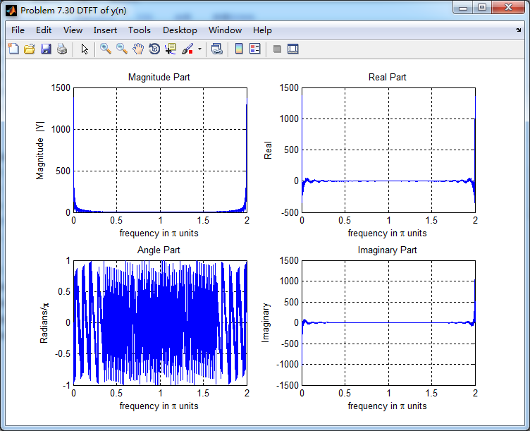
xlabel('frequency in \pi units'); ylabel('Imaginary');

figure('NumberTitle', 'off', 'Name', 'Problem 7.30 DTFT of y(n)')
set(gcf,'Color','white');
subplot(2,2,1); plot(w1/pi,magY); grid on; %axis([0,2,0,15]);
title('Magnitude Part');
xlabel('frequency in \pi units'); ylabel('Magnitude  |Y|');
subplot(2,2,3); plot(w1/pi, angY/pi); grid on; axis([0,2,-1,1]);
title('Angle Part');
xlabel('frequency in \pi units'); ylabel('Radians/\pi');

subplot('2,2,2'); plot(w1/pi, realY); grid on;
title('Real Part');
xlabel('frequency in \pi units'); ylabel('Real');
subplot('2,2,4'); plot(w1/pi, imagY); grid on;
title('Imaginary Part');
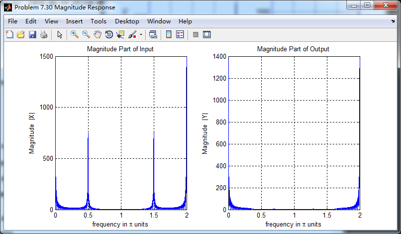
xlabel('frequency in \pi units'); ylabel('Imaginary');

figure('NumberTitle', 'off', 'Name', 'Problem 7.30 Magnitude Response')
set(gcf,'Color','white');
subplot(1,2,1); plot(w1/pi,magX); grid on; %axis([0,2,0,15]);
title('Magnitude Part of Input');
xlabel('frequency in \pi units'); ylabel('Magnitude  |X|');
subplot(1,2,2); plot(w1/pi,magY); grid on; %axis([0,2,0,15]);
title('Magnitude Part of Output');
xlabel('frequency in \pi units'); ylabel('Magnitude  |Y|');

　　运行结果：

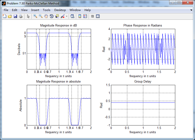
滤波器长度M=47，阻带衰减满足设计指标。

幅度谱和相位谱

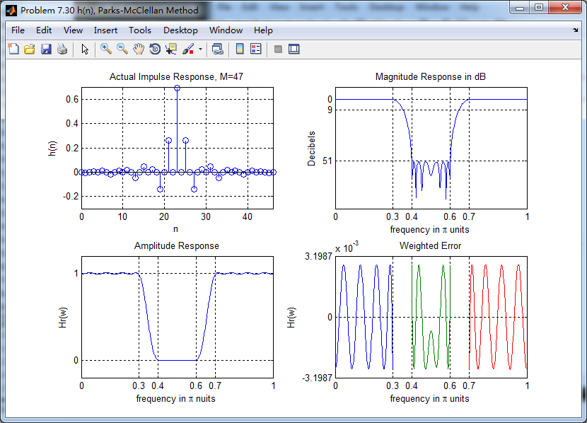
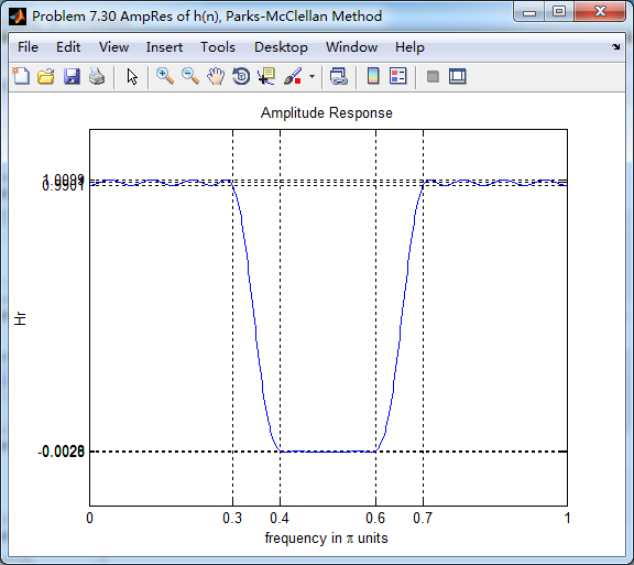
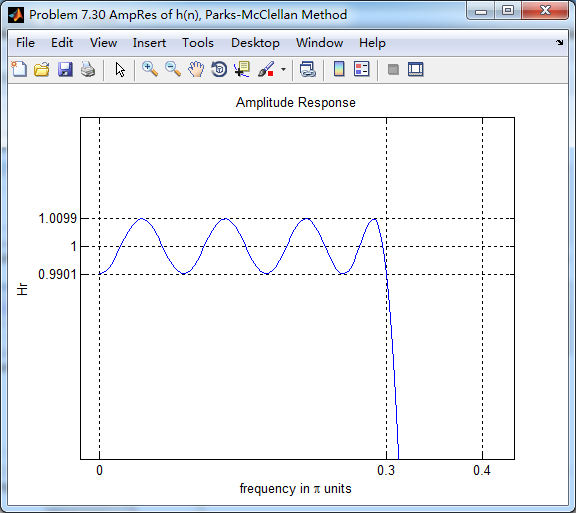
振幅谱，把阻带、通带放大，数数极值点的个数。

下图，9个极值点

下图，8个极值点

下图，9个极值点

总共有9+8+9=26个极值点，M=47，L=(M-1)/2=23，0到π上，最多L+3=26个极值点。

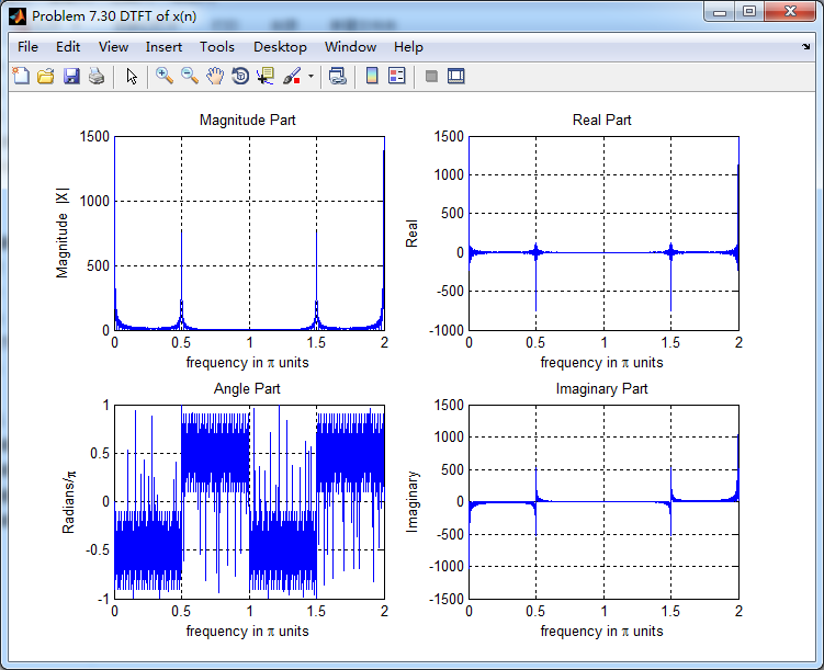
输入输出序列

输入序列的谱，注意0.5π的频率分量，通过带阻滤波后消除了。

输出序列的谱，0.5π分量滤除了。

滤波前后幅度谱对比