26 THINGS I LEARNED IN THE DEEP LEARNING SUMMER SCHOOL

26 THINGS I LEARNED IN THE DEEP LEARNING SUMMER SCHOOL

In the beginning of August I got the chance to attend the Deep Learning Summer School in Montreal. It consisted of 10 days of talks from some of the most well-known neural network researchers. During this time I learned a lot, way more than I could ever fit into a blog post. Instead of trying to pass on 60 hours worth of neural network knowledge, I have made a list of small interesting nuggets of information that I was able to summarise in a paragraph.

At the moment of writing, the summer school website is still online, along with all the presentation slides. All of the information and most of the illustrations come from these slides and are the work of their original authors. The talks in the summer school were filmed as well, hopefully they will also find their way to the web.

Alright, let’s get started.

1. The need for distributed representations

During his first talk, Yoshua Bengio said “This is my most important slide”. You can see that slide below: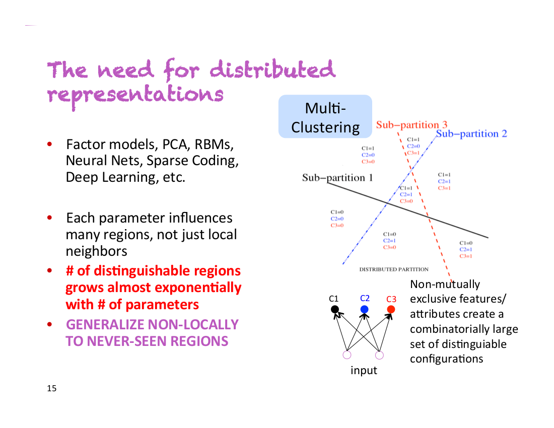

Let’s say you have a classifier that needs to detect people that are male/female, have glasses or don’t have glasses, and are tall/short. With non-distributed representations, you are dealing with 2*2*2=8 different classes of people. In order to train an accurate classifier, you need to have enough training data for each of these 8 classes. However, with distributed representations, each of these properties could be captured by a different dimension. This means that even if your classifier has never encountered tall men with glasses, it would be able to detect them, because it has learned to detect gender, glasses and height independently from all the other examples.

2. Local minima are not a problem in high dimensions

The team of Yoshua Bengio have experimentally found that when optimising the parameters of high-dimensional neural nets, there effectively are no local minima. Instead, there are saddle points which are local minima in some dimensions but not all. This means that training can slow down quite a lot in these points, until the network figures out how to escape, but as long as we’re willing to wait long enough then it will find a way.

Below is a graph demonstrating a network during training, oscillating between two states: approaching a saddle point and then escaping it.

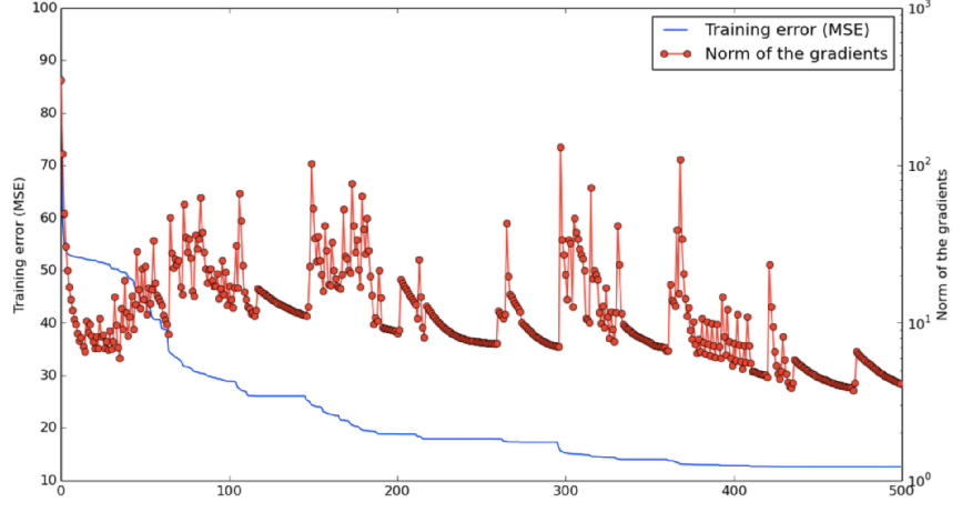
Given one specific dimension, there is some small probability p with which a point is a local minimum, but not a global minimum, in that dimension. Now, the probability of a point in a 1000-dimensional space being an incorrect local minimum in all of these would be p1000, which is just astronomically small. However, the probability of it being a local minimum in some of these dimensions is actually quite high. And when we get these minima in many dimensions at once, then training can appear to be stuck until it finds the right direction.

In addition, this probability p will increase as the loss function gets closer to the global minimum.  This means that if we do ever end up at a genuine local minimum, then for all intents and purposes it will be close enough to the global minimum that it will not matter.

3. Derivatives derivatives derivatives

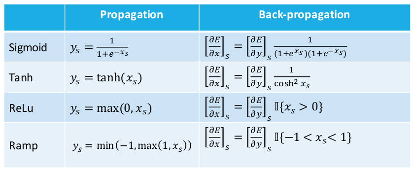
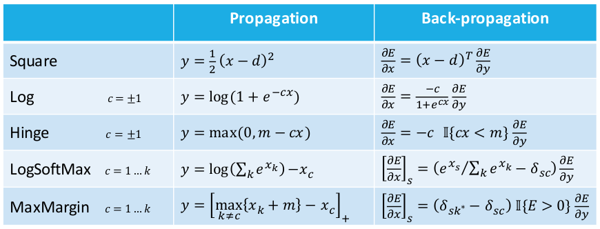
Leon Bottou had some useful tables with activation functions, loss functions, and their corresponding derivatives. I’ll keep these here for later.

4. Weight initialisation strategy

The current recommended strategy for initialising weights in a neural network is to sample values W(k)i,j uniformly from [−b,b], where

b=6Hk+Hk+1−−−−−−√

Hk and Hk+1 are the sizes of hidden layers before and after the weight matrix.

Recommended by Hugo Larochelle, published by Glorot & Bengio (2010).

5. Neural net training tricks

A few practical suggestions from Hugo Larochelle:

• Normalise real-valued data. Subtract the mean and divide by standard deviation.
• Decrease the learning rate during training.
• Can update using mini-batches – the gradient is more stable.
• Can use momentum, to get through plateaus.

6. Gradient checking

If you implemented your backprop by hand and it’s not working, then there’s roughly 99% chance that the gradient calculation has a bug. Use gradient checking to identify the issue. The idea is to use the definition of a gradient: how much will the model error change, if we increase a specific weight by a small amount.

∂f(x)∂x≈f(x+ϵ)–f(x−ϵ)2ϵ

A more in-depth explanation is available here: Gradient checking and advanced optimization

7. Motion tracking

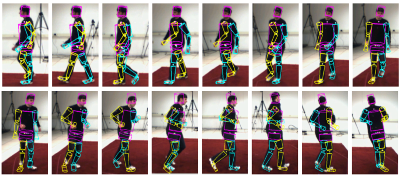
Human motion tracking can be done with impressive accuracy. Below are examples from the paper Dynamical Binary Latent Variable Models for 3D Human Pose Tracking by Graham Taylor et al. (2010). The method uses conditional restricted Boltzmann machines.

8. Syntax or no syntax? (aka, “is syntax a thing?”)

Chris Manning and Richard Socher have put a lot of effort into developing compositional models that combine neural embeddings with more traditional parsing approaches. This culminated with a Recursive Neural Tensor Network (Socher et al., 2013), which uses both additive and multiplicative interactions to combine word meanings along a parse tree.

And then, the model was beaten (by quite a margin) by the Paragraph Vector (Le & Mikolov, 2014), which knows absolutely nothing about the sentence structure or syntax. Chris Manning referred to this result as “a defeat for creating ‘good’ compositional vectors”.

However, more recent work using parse trees has again surpassed this result. Irsoy & Cardie (NIPS, 2014) managed to beat paragraph vectors by going “deep” with their networks in multiple dimensions. Finally, Tai et al. (ACL, 2015) have improved the results again by combining LSTMs with parse trees.

The accuracies of these models on the Stanford 5-class sentiment dataset are as follows:

Method	Accuracy
RNTN (Socher et al. 2013)	45.7
Paragraph Vector (Le & Mikolov 2014)	48.7
DRNN (Irsoy & Cardie 2014)	49.8
Tree LSTM (Tai et al. 2015)	50.9

So it seems that, at the moment, models using the parse tree are beating simpler approaches. I’m curious to see if and when the next syntax-free approach will emerge that will advance this race. After all, the goal of many neural models is not to discard the underlying grammar, but to implicitly capture it in the same network.

9. Distributed vs distributional

Chris Manning himself cleared up the confusion between the two words.

Distributed: A concept is represented as continuous activation levels in a number of elements. Like a dense word embedding, as opposed to 1-hot vectors.

Distributional: Meaning is represented by contexts of use. Word2vec is distributional, but so are count-based word vectors, as we use the contexts of the word to model the meaning.

10. The state of dependency parsing

Comparison of dependency parsers on the Penn Treebank:

Parser	Unlabelled Accuracy	Labelled Acccuracy	Speed (sent/s)
MaltParser	89.8	87.2	469
MSTParser	91.4	88.1	10
TurboParser	92.3	89.6	8
Stanford Neural Dependency Parser	92.0	89.7	654
Google	94.3	92.4	?

The last result is from Google “pulling out all the stops”, by putting massive amounts of resources into training the Stanford neural parser.

11. Theano

Well, I knew a bit about Theano before, but I learned a whole lot more during the summer school. And it is pretty awesome.

Since Theano originates from Montreal, it was especially helpful to be able to ask questions directly from the people who are developing it.

Most of the information that was presented is available online, in the form of interactive python tutorials.

12. Nvidia Digits

Nvidia has a toolkit called Digits that trains and visualises complex neural network models without needing to write any code. And they’re selling DevBox – a machine customised for running Digits and other deep learning software (Theano, Caffe, etc). It comes with 4 Titan X GPUs and currently costs $15,000.

13. Fuel

Fuel is a toolkit that manages iteration over your datasets – it can split them into minibatches, manage shuffling, apply various preprocessing steps, etc. There are prebuilt functions for some established datasets, such as MNIST, CIFAR-10, and Google’s 1B Word corpus. It is mainly designed for use with Blocks, a toolkit that simplifies network construction with Theano.

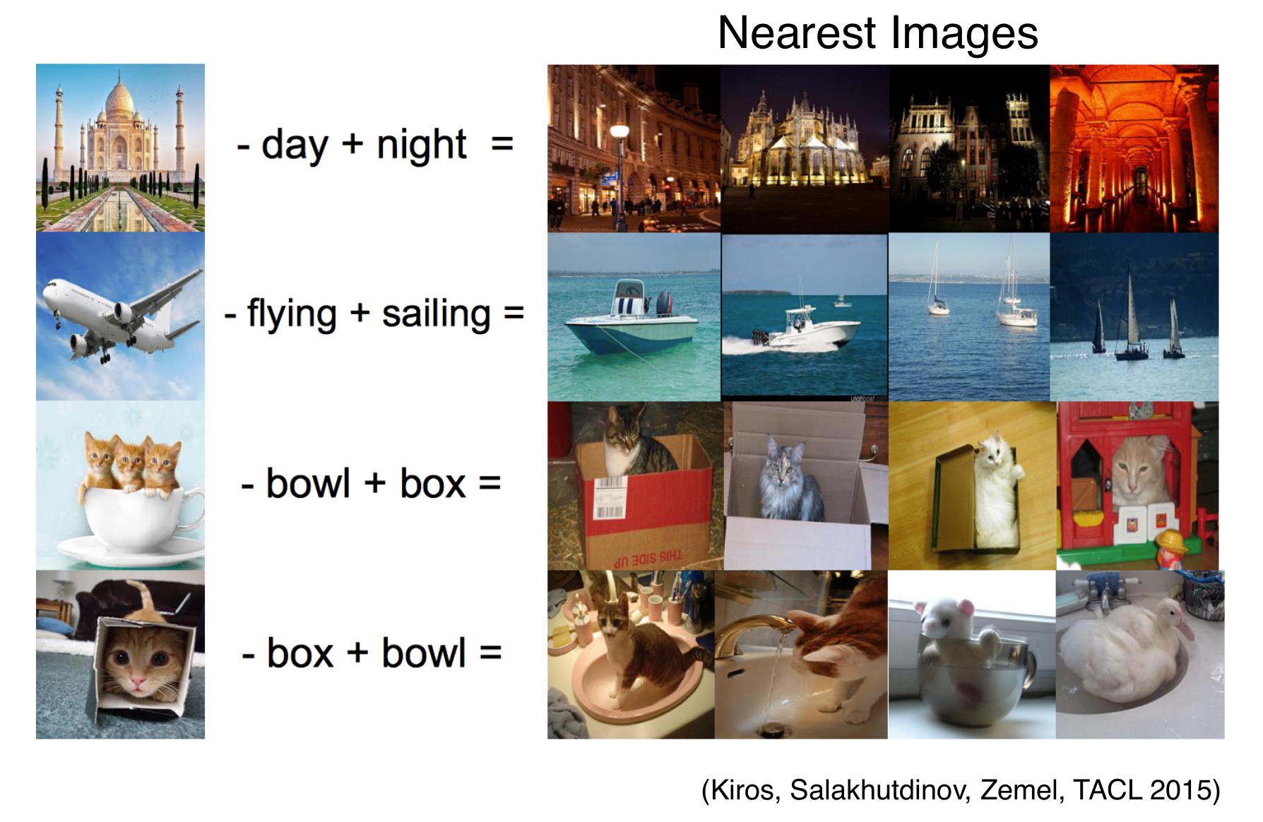
14. Multimodal linguistic regularities

Remember “king – man + woman = queen”? Turns out that works with images as well (Kiros et al., 2015).

15. Taylor series approximation

When we are at point x0 and take a step to x, then we can estimate the function value in the new location by knowing the derivatives, using the Taylor series approximation.

f(x)=f(x0)+(x–x0)f′(x)+12(x–x0)2f”(x)+…

Similarly, we can estimate the loss of a function, when we update parameters θ0 to θ.

J(θ)=J(θ0)+(θ–θ0)Tg+12(x–x0)TH(x–x0)+…

where g contains the derivatives with respect to θ, and H is the Hessian with second order derivatives with respect to θ.

This is the second-order Taylor approximation, but we could increase the accuracy by adding even higher-order derivatives.

16. Computational intensity

Adam Coates presented a strategy for analysing the speed of matrix operations on a GPU. It’s a simplified model that says your time is spent on either reading/writing to memory or doing calculations. It assumes you can do both in parallel so we are interested in which one of them takes more time.

Let’s say we are multiplying a matrix with a vector:

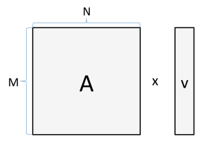
If M=1024 and N=512, then the number of bytes we need to read and store is:

4 bytes ×(1024×512+512+1024)=2.1e6 bytes

And the number of calculations we need to do is:

2×1024×512=1e6 FLOPs

If we have a GPU that can do 6 TFLOP/s and has memory bandwidth of  300GB/s, then the total running time will be:

max{2.1e6 bytes /(300e9 bytes/s),1e6 FLOPs/(6e12 FLOP/s)}=max{7μs,0.16μs}

This means the process is bounded by the 7μs spent on copying to/from the memory, and getting a faster GPU would not make any difference. As you can probably guess, this situation gets better with bigger matrices/vectors, and when doing matrix-matrix operations.

Adam also described the idea of calculating the intensity of an operation:

Intensity = (# arithmetic ops) / (# bytes to load or store)

In the previous scenario, this would be

Intensity = (1E6 FLOPs) / (2.1E6 bytes) = 0.5 FLOPs/bytes

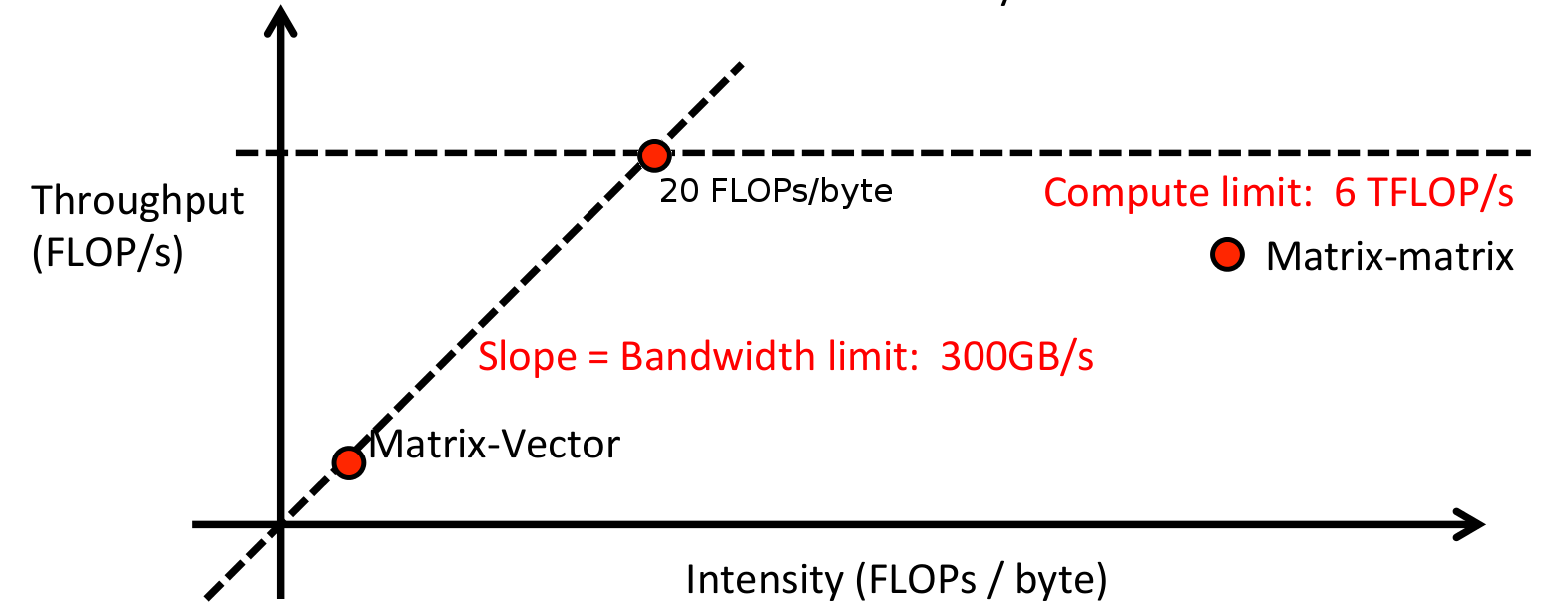
Low intensity means the system is bottlenecked on memory, and high intensity means it’s bottlenecked by the GPU speed. This can be visualised, in order to find which of the two needs to improve in order to speed up the whole system, and where the sweet spot lies.

17. Minibatches

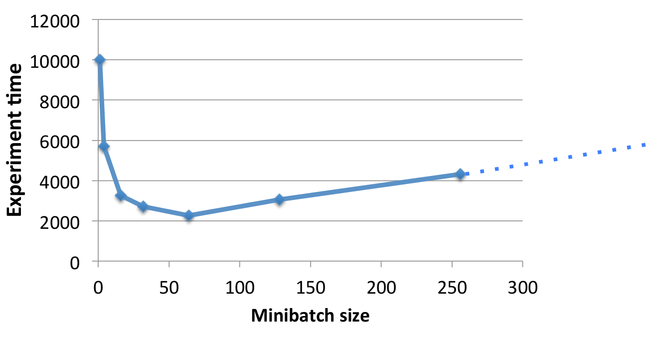
Continuing from the intensity calculations, one way of increasing the intensity of your network (in order to be limited by computation instead of memory), is to process data in minibatches. This avoids some memory operations, and GPUs are great at processing large matrices in parallel.

However, increasing the batch size too much will probably start to hurting the training algorithm and converging can take longer. It’s important to find a good balance in order to get the best results in the least amount of time.

18. Training on adversarial examples

It was recently revealed that neural networks are easily tricked by adversarial examples. In the example below, the image on the left is correctly classified as a goldfish. However, if we apply the noise pattern shown in the middle, resulting in the image on the right, the classifier becomes convinced this is a picture of a daisy. The image is from Andrej Karpathy’s blog post “Breaking Linear Classifiers on ImageNet”, and you can read more about it there.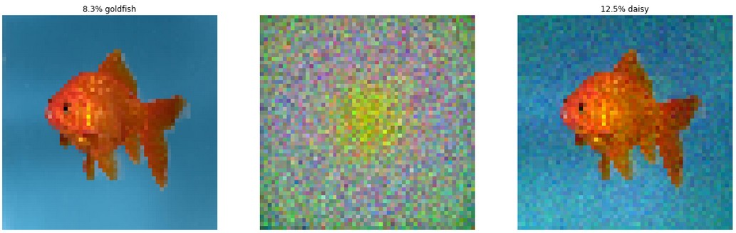 

The noise pattern isn’t random though – the noise is carefully calculated, in order to trick the network. But the point remains: the image on the right is clearly still a goldfish and not a daisy.

Apparently strategies like ensemble models, voting after multiple saccades, and unsupervised pretraining have all failed against this vulnerability. Applying heavy regularisation helps, but not before ruining the accuracy on the clean data.

Ian Goodfellow presented the idea of training on these adversarial examples. They can be automatically generated and added to the training set. The results below show that in addition to helping with the adversarial cases, this also improves accuracy on the clean examples.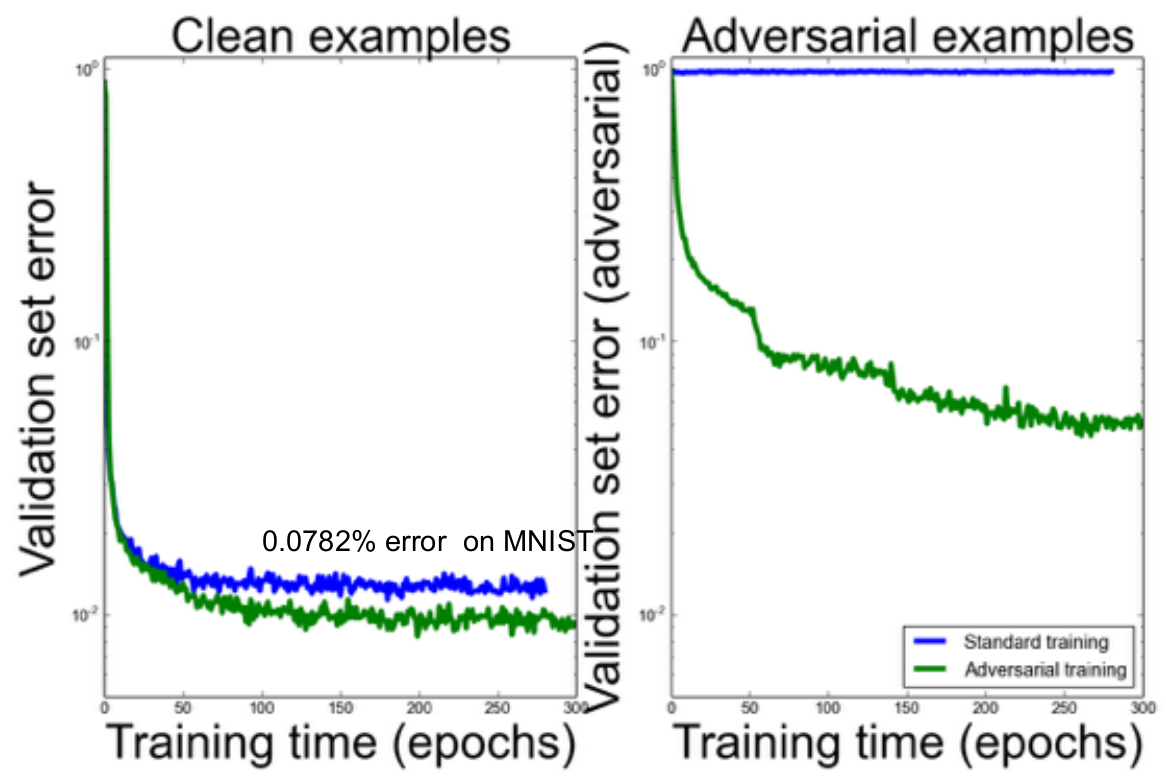Finally, we can improve this further by penalising the KL-divergence between the original predicted distribution and the predicted distribution on the adversarial example. This optimises the network to be more robust, and to predict similar class distributions for similar (adversarial) images.

19. Everything is language modelling

Phil Blunsom presented the idea that almost all NLP can be structured as a language model. We can do this by concatenating the output to the input and trying to predict the probability of the whole sequence.

Translation:

P(Les chiens aiment les os || Dogs love bones)

Question answering:

P(What do dogs love? || bones .)

Dialogue:

P(How are you? || Fine thanks. And you?)

The latter two need to be additionally conditioned on some world knowledge. The second part doesn’t even need to be words, but could be labels or some structured output like dependency relations.

20. SMT had a rough start

When Frederick Jelinek and his team at IBM submitted one of the first papers on statistical machine translation to COLING in 1988, they got the following anonymous review:

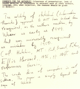
The validity of a statistical (information theoretic) approach to MT has indeed been recognized, as the authors mention, by Weaver as early as 1949. And was universally recognized as mistaken by 1950 (cf. Hutchins, MT – Past, Present, Future, Ellis Horwood, 1986, p. 30ff and references therein). The crude force of computers is not science. The paper is simply beyond the scope of COLING.

21. The state of Neural Machine Translation

Apparently a very simple neural model can produce surprisingly good results. An example of translating from Chinese to English, from Phil Blunsom’s slides:

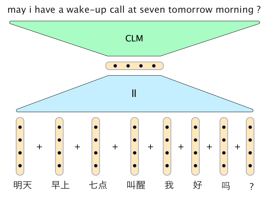
In this model, the vectors for the Chinese words are simply added together to form a sentence vector. The decoder consists of a conditional language model which takes the sentence vector, together with vectors from the two recently generated English words, and generates the next word in the translation.

However, neural models are still not outperforming the very best traditional MT systems. They do come very close though. Results from“Sequence to Sequence Learning with Neural Networks” by Sutskever et al. (2014):

Model	BLEU score
Baseline	33.30
Best WMT'14 result	37.0
Scoring with 5 LSTMs	36.5
Oracle (upper bound)	∼45

22. MetaMind classifier demo

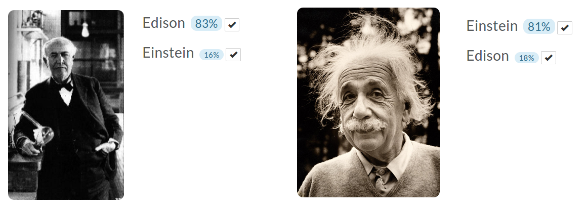
Richard Socher demonstrated the MetaMind image classification demo, which you can train yourself by uploading images. I trained a classifier to detect Edison and Einstein (couldn’t find enough unique images of Tesla). 5 example images for both classes, testing on one held out image each. Seemed to work pretty well.

23. Optimising gradient updates

Mark Schmidt gave two presentations about numerical optimisation in different scenarios.

In a deterministic gradient method we calculate the gradient over the whole dataset and then apply the update. The iteration cost is linear with the dataset size.

In stochastic gradient methods we calculate the gradient on one datapoint and then apply the update. The iteration cost is independent of the dataset size.

Each iteration of the stochastic gradient descent is much faster, but it usually takes many more iterations to train the network, as this graph illustrates:

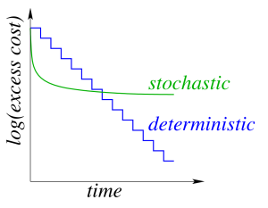
In order to get the best of both worlds, we can use batching. More specifically, we could do one pass of the dataset with stochastic gradient descent, in order to quickly get on the right track, and then start increasing the batch size. The gradient error decreases as the batch size increases, although eventually the iteration cost will become dependent on the dataset size again.

Stochastic Average Gradient (SAG) is a method that gets around this, providing a linear convergence rate with only 1 gradient per iteration. Unfortunately, it is not feasible for large neural networks, as it needs to remember the gradient updates for every datapoint, leading to large memory requirements. Stochastic Variance-Reduced Gradient (SVRG) is another method that reduces the memory cost, but only needs 2 gradient calculations per iteration (plus occasional full passes).

Mark said a student of his implemented a variety of optimisation methods (AdaGrad, momentum, SAG, etc). When asked, what he would use in a black box neural network system, the student said two methods: Streaming SVRG(Frostig et al., 2015), and a method they haven’t published yet.

24. Theano profiling

If you put “profile=True” into THEANO_FLAGS, it will analyse your program, showing a breakdown of how much is spent on each operation. Very handy for finding bottlenecks.

25. Adversarial nets framework

Following on from Ian Goodfellow’s talk on adversarial examples, Yoshua Bengio talked about having two systems competing with each other.

System D is a discriminative system that aims to classify between real data and artificially generated data.

System G is a generative system, that tries to generate artificial data, which D would incorrectly classify as real.

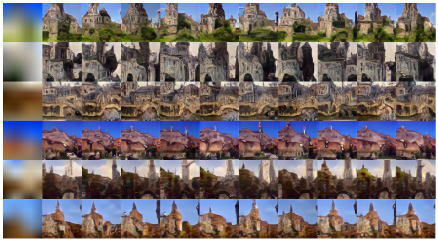
As we train one, the other needs to get better as well. In practice this does work, although the step needs to be quite small to make sure D can keep up with G. Below are some examples from “Deep Generative Image Models using a Laplacian Pyramid of Adversarial Networks” – a more advanced version of this model which tries to generate images of churches.

26. arXiv.org numbering

The arXiv number contains the year and month of the submission, followed by the sequence number. So paper 1508.03854 was number 3854 in August 2015. Good to know.