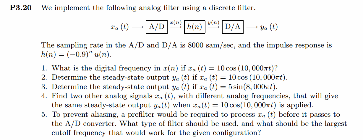
《DSP using MATLAB》Problem 3.20

代码：

%% ------------------------------------------------------------------------
%%            Output Info about this m-file
fprintf('\n***********************************************************\n');
fprintf('        <DSP using MATLAB> Problem 3.20 \n\n');

banner();
%% ------------------------------------------------------------------------

%% -------------------------------------------------------------------
%%                     xa(t)=10cos(10000πt)  through A/D
%% -------------------------------------------------------------------
Fs = 8000;                       % sample/sec
Ts = 1/Fs;                       % sample interval, 0.125ms=0.000125s

n1_start = -80; n1_end = 80;
      n1 = [n1_start:1:n1_end];
     nTs = n1 * Ts;              % [-10,10]ms    [-0.01,0.01]s

x1 = 10*cos(10000*pi*nTs);       % Digital signal

M = 500;
[X1, w] = dtft1(x1, n1, M);

magX1  = abs(X1);  angX1  = angle(X1);  realX1  = real(X1);  imagX1  = imag(X1);

%% --------------------------------------------------------------------
%%              START X(w)'s  mag ang real imag
%% --------------------------------------------------------------------
figure('NumberTitle', 'off', 'Name', 'Problem 3.20 X1');
set(gcf,'Color','white');
subplot(2,1,1); plot(w/pi,magX1); grid on;  %axis([-1,1,0,1.05]);
title('Magnitude Response');
xlabel('frequency in \pi units'); ylabel('Magnitude  |H|');
subplot(2,1,2); plot(w/pi, angX1/pi); grid on;  %axis([-1,1,-1.05,1.05]);
title('Phase Response');
xlabel('frequency in \pi units'); ylabel('Radians/\pi');

figure('NumberTitle', 'off', 'Name', 'Problem 3.20 X1');
set(gcf,'Color','white');
subplot(2,1,1); plot(w/pi, realX1); grid on;
title('Real Part');
xlabel('frequency in \pi units'); ylabel('Real');
subplot(2,1,2); plot(w/pi, imagX1); grid on;
title('Imaginary Part');
xlabel('frequency in \pi units'); ylabel('Imaginary');
%% -------------------------------------------------------------------
%%             END X's  mag ang real imag
%% -------------------------------------------------------------------

%% --------------------------------------------------------
%%                    h(n) = (-0.9)^n[u(n)]
%% --------------------------------------------------------
n2 = n1;
h = (-0.9) .^ (n2) .* stepseq(0, n1_start, n1_end);

figure('NumberTitle', 'off', 'Name', 'Problem 3.20 h(n)');
set(gcf,'Color','white');
%subplot(2,1,1);
stem(n2, h); grid on;  %axis([-1,1,0,1.05]);
title('Impulse Response: (-0.9)^n[u(n)]');
xlabel('n'); ylabel('h');

[H, w] = dtft1(h, n2, M);

magH  = abs(H);  angH  = angle(H);  realH  = real(H);  imagH  = imag(H);

%% --------------------------------------------------------------------
%%              START H(w)'s  mag ang real imag
%% --------------------------------------------------------------------
figure('NumberTitle', 'off', 'Name', 'Problem 3.20 H');
set(gcf,'Color','white');
subplot(2,1,1); plot(w/pi,magH); grid on;  %axis([-1,1,0,1.05]);
title('Magnitude Response');
xlabel('frequency in \pi units'); ylabel('Magnitude  |H|');
subplot(2,1,2); plot(w/pi, angH/pi); grid on;  %axis([-1,1,-1.05,1.05]);
title('Phase Response');
xlabel('frequency in \pi units'); ylabel('Radians/\pi');

figure('NumberTitle', 'off', 'Name', 'Problem 3.20 H');
set(gcf,'Color','white');
subplot(2,1,1); plot(w/pi, realH); grid on;
title('Real Part');
xlabel('frequency in \pi units'); ylabel('Real');
subplot(2,1,2); plot(w/pi, imagH); grid on;
title('Imaginary Part');
xlabel('frequency in \pi units'); ylabel('Imaginary');
%% -------------------------------------------------------------------
%%             END X's  mag ang real imag
%% -------------------------------------------------------------------

%% ----------------------------------------------
%%                 y(n)=x(n)*h(n)
%% ----------------------------------------------
[y, ny] = conv_m(x1, n1, h, n1);

figure('NumberTitle', 'off', 'Name', 'Problem 3.20 y(n)');
set(gcf,'Color','white');
%subplot(2,1,1);
stem(ny, y); grid on;  %axis([-1,1,0,1.05]);
title('x(n)*h(n)');
xlabel('n'); ylabel('y');

[Y, w] = dtft1(y, ny, M);

magY  = abs(Y);  angY  = angle(Y);  realY  = real(Y);  imagY  = imag(Y);

%% --------------------------------------------------------------------
%%              START Y(w)'s  mag ang real imag
%% --------------------------------------------------------------------
figure('NumberTitle', 'off', 'Name', 'Problem 3.20 Y');
set(gcf,'Color','white');
subplot(2,1,1); plot(w/pi,magY); grid on;  %axis([-1,1,0,1.05]);
title('Magnitude Response');
xlabel('frequency in \pi units'); ylabel('Magnitude  |H|');
subplot(2,1,2); plot(w/pi, angY/pi); grid on;  %axis([-1,1,-1.05,1.05]);
title('Phase Response');
xlabel('frequency in \pi units'); ylabel('Radians/\pi');

figure('NumberTitle', 'off', 'Name', 'Problem 3.20 Y');
set(gcf,'Color','white');
subplot(2,1,1); plot(w/pi, realY); grid on;
title('Real Part');
xlabel('frequency in \pi units'); ylabel('Real');
subplot(2,1,2); plot(w/pi, imagY); grid on;
title('Imaginary Part');
xlabel('frequency in \pi units'); ylabel('Imaginary');
%% -------------------------------------------------------------------
%%             END X's  mag ang real imag
%% -------------------------------------------------------------------

%% ----------------------------------------------------------
%%                  xa(t) reconstruction from x1(n)
%% ----------------------------------------------------------

Dt = 0.00005; t = -0.01:Dt:0.01;
xa = x1 * sinc(Fs*(ones(length(n1),1)*t - nTs'*ones(1,length(t)))) ;

figure('NumberTitle', 'off', 'Name', 'Problem 3.20 Reconstructed From x1(n)');
set(gcf,'Color','white');
%subplot(2,1,1);
stairs(nTs*1000,x1); grid on;  %axis([0,1,0,1.5]);       % Zero-Order-Hold
title('Reconstructed Signal from x1(n) using zero-order-hold');
xlabel('t in msec.'); ylabel('xa(t)'); hold on;
stem(nTs*1000, x1); gtext('ZOH'); hold off;

figure('NumberTitle', 'off', 'Name', 'Problem 3.20 Reconstructed From x1(n)');
set(gcf,'Color','white');
%subplot(2,1,2);
plot(nTs*1000,x1); grid on;  %axis([0,1,0,1.5]);       % first-Order-Hold
title('Reconstructed Signal from x1(n) using first-Order-Hold');
xlabel('t in msec.'); ylabel('xa(t)'); hold on;
stem(nTs*1000,x1); gtext('FOH'); hold off;

xa = spline(nTs, x1, t);
figure('NumberTitle', 'off', 'Name', sprintf('Problem 3.20 Ts = %.6fs', Ts));
set(gcf,'Color','white');
%subplot(2,1,1);
plot(1000*t, xa);
xlabel('t in ms units'); ylabel('x');
title(sprintf('Reconstructed Signal from x1(n) using spline function')); grid on; hold on;
stem(1000*nTs, x1); gtext('spline');

%% ----------------------------------------------------------------
%%                     y(n) through D/A, reconstruction
%% ----------------------------------------------------------------
Dt = 0.00005; t = -0.02:Dt:0.02;
ya = y * sinc(Fs*(ones(length(ny),1)*t - (ny*Ts)'*ones(1,length(t)))) ;

figure('NumberTitle', 'off', 'Name', 'Problem 3.20 Reconstructed From y(n)');
set(gcf,'Color','white');
%subplot(2,1,1);
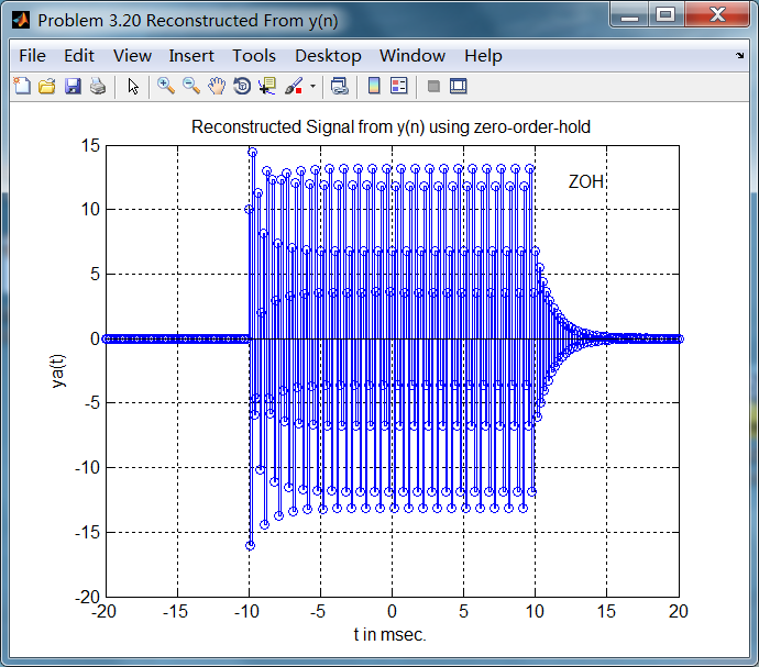
stairs(ny*Ts*1000,y); grid on;  %axis([0,1,0,1.5]);       % Zero-Order-Hold
title('Reconstructed Signal from y(n) using zero-order-hold');
xlabel('t in msec.'); ylabel('ya(t)'); hold on;
stem(ny*Ts*1000, y); gtext('ZOH'); hold off;

figure('NumberTitle', 'off', 'Name', 'Problem 3.20 Reconstructed From y(n)');
set(gcf,'Color','white');
%subplot(2,1,2);
plot(ny*Ts*1000,y); grid on;  %axis([0,1,0,1.5]);       % first-Order-Hold
title('Reconstructed Signal from y(n) using first-Order-Hold');
xlabel('t in msec.'); ylabel('ya(t)'); hold on;
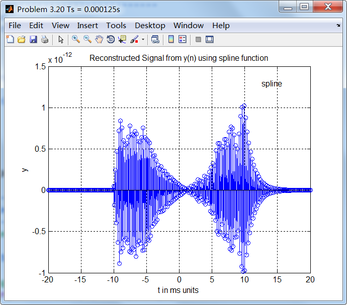
stem(ny*Ts*1000,y); gtext('FOH'); hold off;

ya = spline(ny*Ts, y, t);
figure('NumberTitle', 'off', 'Name', sprintf('Problem 3.20 Ts = %.6fs', Ts));
set(gcf,'Color','white');
%subplot(2,1,1);
plot(1000*t, ya);
xlabel('t in ms units'); ylabel('y');
title(sprintf('Reconstructed Signal from y(n) using spline function')); grid on; hold on;
stem(1000*ny*Ts, y); gtext('spline');

　　运行结果：

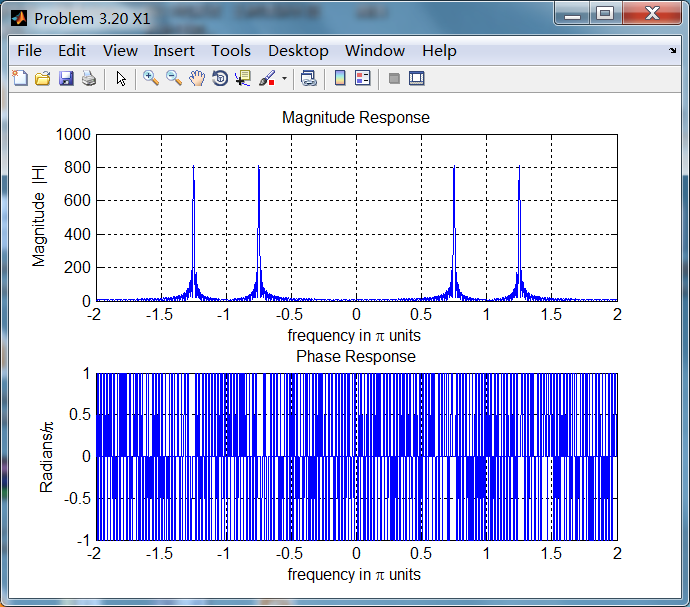
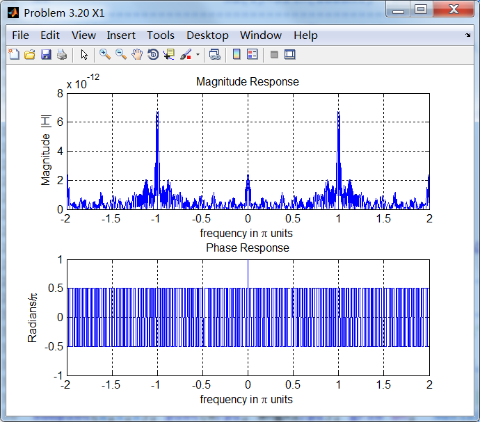
2、模拟信号经过Fs=8000sample/sec采样后，得采样信号的谱，如下图，0.75π处为假频。

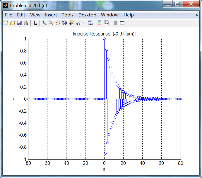
脉冲响应序列如下：

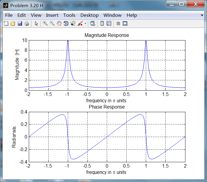
系统的频率响应，即脉冲响应序列的DTFT：

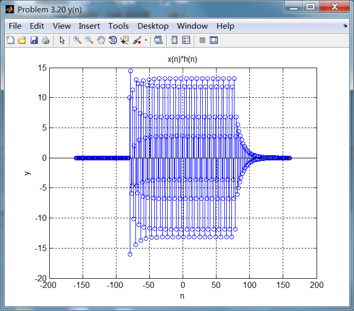
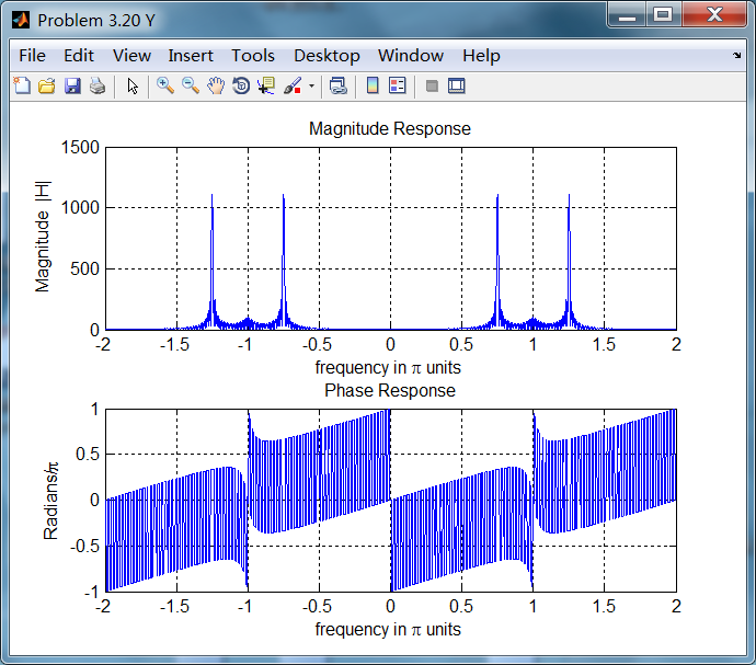
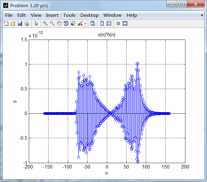
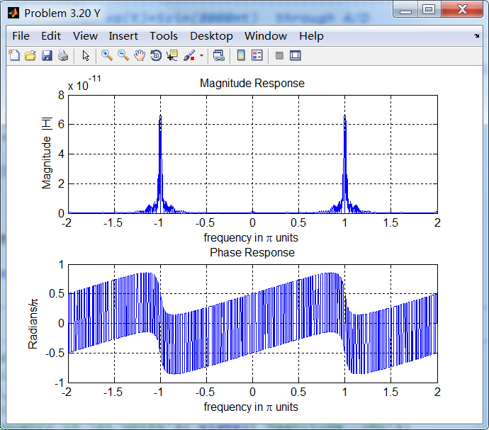
输出信号及其DTFT：

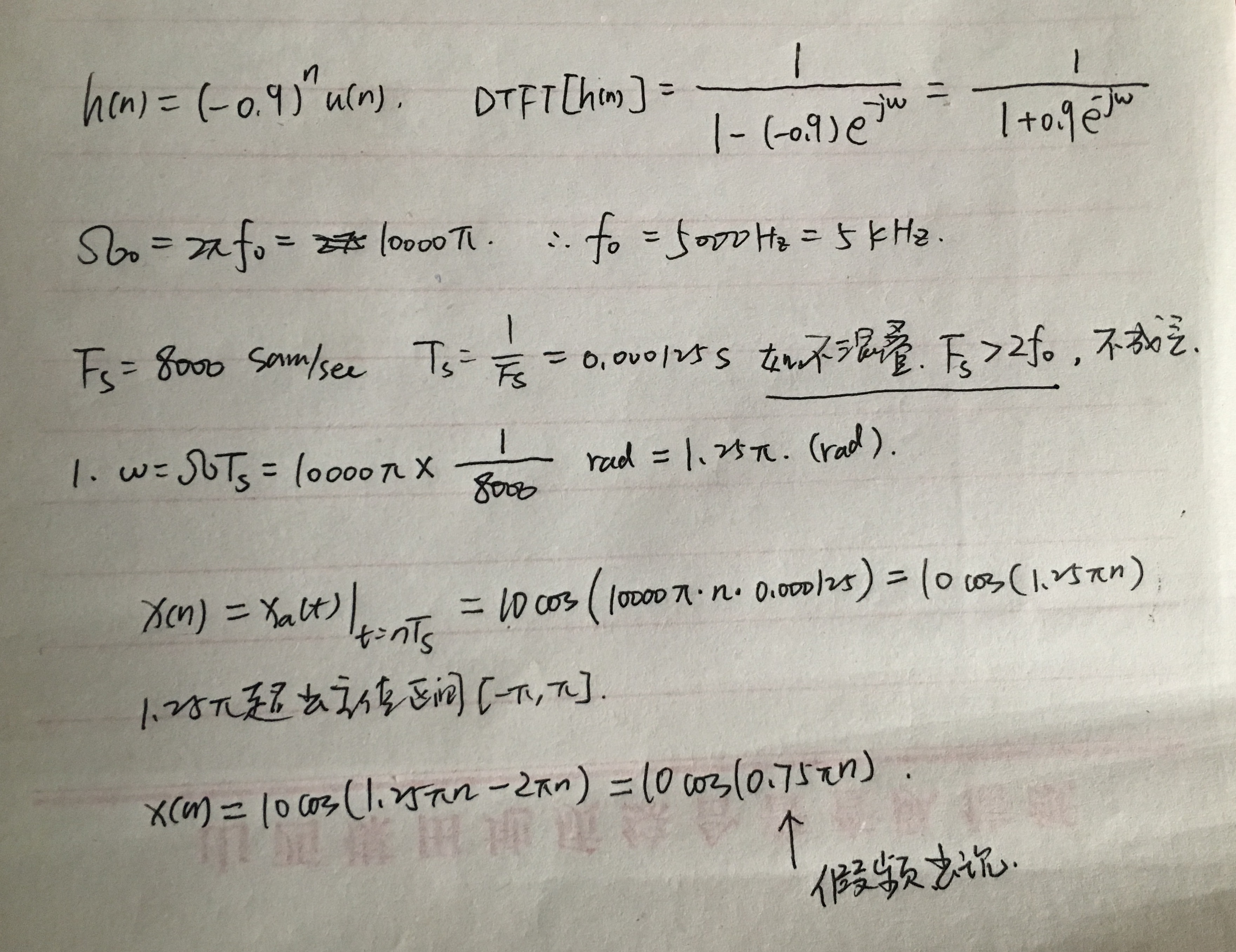
3、第3小题中的模拟信号经Fs=8000采样后，数字角频率为π，

采样后信号的谱：

采样后信号经过滤波器，输出信号的谱，

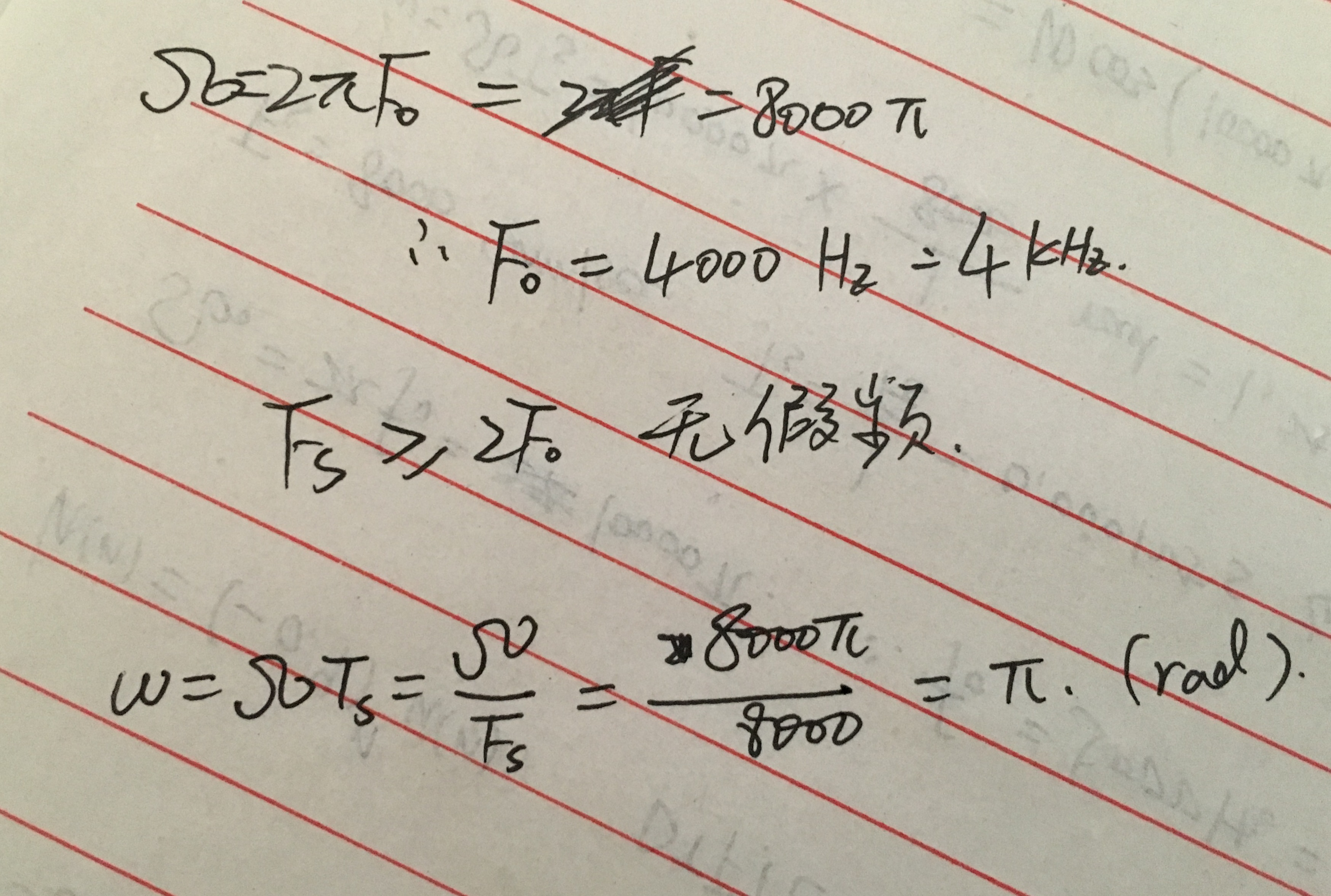
4、找到另外两个不同的模拟角频率的模拟信号，使得采样后和第1小题模拟信号采样后稳态输出相同。

想求的数字角频率和第1题的数字角频率0.75π+2π，对应的模拟频率如下计算：

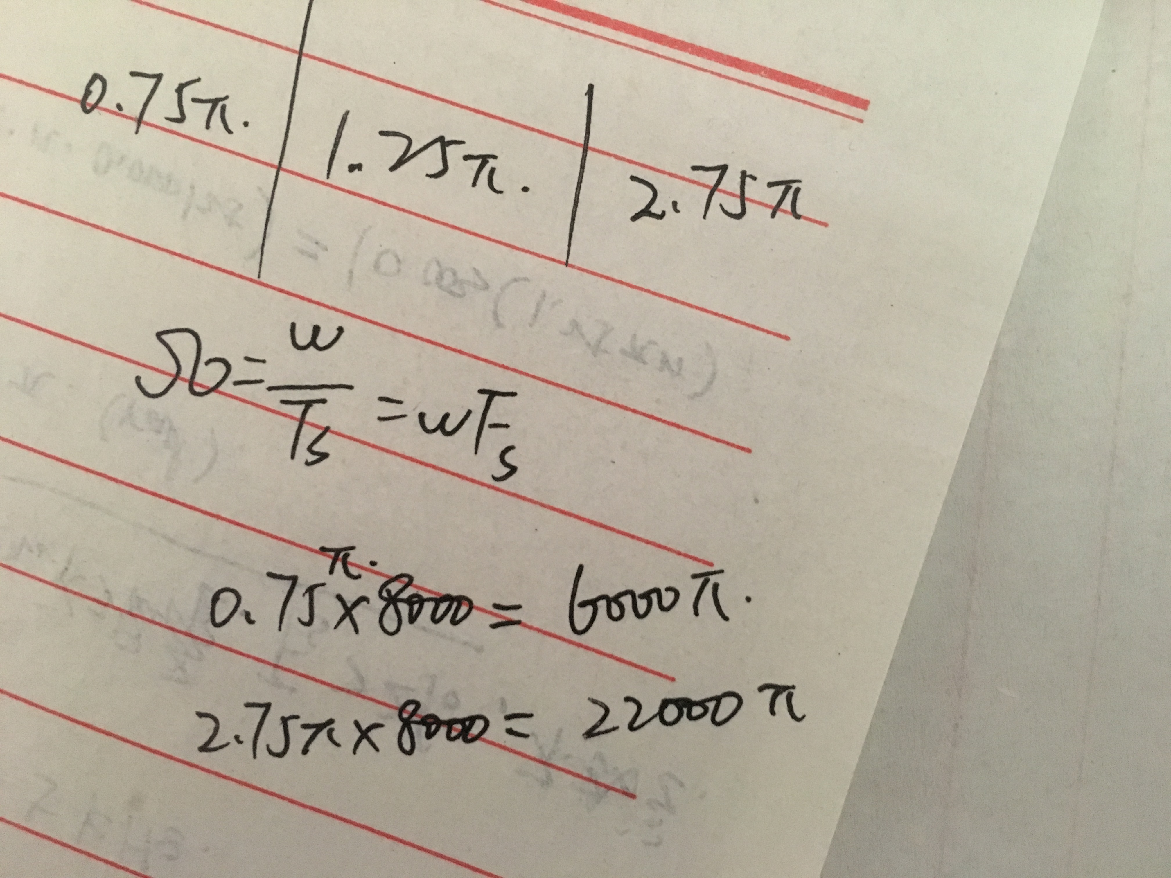
5、根据抽样定理，采用截止频率F0=4kHz，低通滤波器。