吴裕雄 数据挖掘与分析案例实战（7）——岭回归与LASSO回归模型

# 导入第三方模块
import pandas as pd
import numpy as np
import matplotlib.pyplot as plt
from sklearn import model_selection
from sklearn.linear_model import Ridge,RidgeCV

# 读取糖尿病数据集
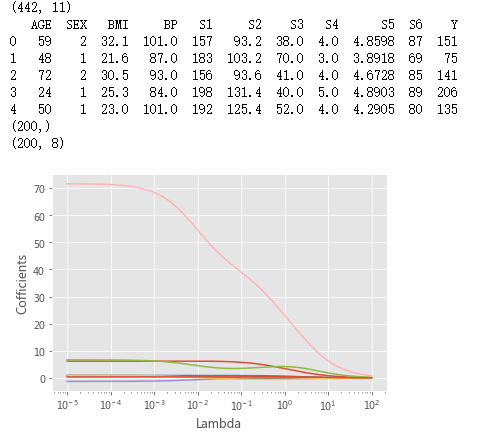
diabetes = pd.read_excel(r'F:\\python_Data_analysis_and_mining\\08\\diabetes.xlsx', sep = '')
print(diabetes.shape)
print(diabetes.head())
# 构造自变量（剔除患者性别、年龄和因变量）
predictors = diabetes.columns[2:-1]
# 将数据集拆分为训练集和测试集
X_train, X_test, y_train, y_test = model_selection.train_test_split(diabetes[predictors], diabetes['Y'],test_size = 0.2, random_state = 1234 )
# 构造不同的Lambda值
Lambdas = np.logspace(-5, 2, 200)
print(Lambdas.shape)
# 构造空列表，用于存储模型的偏回归系数
ridge_cofficients = []
# 循环迭代不同的Lambda值
for Lambda in Lambdas:
ridge = Ridge(alpha = Lambda, normalize=True)
ridge.fit(X_train, y_train)
ridge_cofficients.append(ridge.coef_)
print(np.shape(ridge_cofficients))
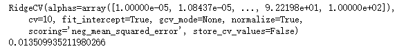
# 绘制Lambda与回归系数的关系
# 中文乱码和坐标轴负号的处理
plt.rcParams['font.sans-serif'] = ['Microsoft YaHei']
plt.rcParams['axes.unicode_minus'] = False
# 设置绘图风格
plt.style.use('ggplot')
plt.plot(Lambdas, ridge_cofficients)
# 对x轴作对数变换
plt.xscale('log')
# 设置折线图x轴和y轴标签
plt.xlabel('Lambda')
plt.ylabel('Cofficients')
# 图形显示
plt.show()

# 岭回归模型的交叉验证
# 设置交叉验证的参数，对于每一个Lambda值，都执行10重交叉验证
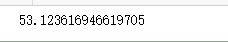
ridge_cv = RidgeCV(alphas = Lambdas, normalize=True, scoring='neg_mean_squared_error', cv = 10)
print(ridge_cv)
# 模型拟合
ridge_cv.fit(X_train, y_train)
# 返回最佳的lambda值
ridge_best_Lambda = ridge_cv.alpha_
print(ridge_best_Lambda)

# 导入第三方包中的函数
from sklearn.metrics import mean_squared_error

# 基于最佳的Lambda值建模
ridge = Ridge(alpha = ridge_best_Lambda, normalize=True)
ridge.fit(X_train, y_train)
# 返回岭回归系数
pd.Series(index = ['Intercept'] + X_train.columns.tolist(),data = [ridge.intercept_] + ridge.coef_.tolist())
# 预测
ridge_predict = ridge.predict(X_test)
# 预测效果验证
RMSE = np.sqrt(mean_squared_error(y_test,ridge_predict))
print(RMSE)

# 导入第三方模块中的函数
from sklearn.linear_model import Lasso,LassoCV

# 构造空列表，用于存储模型的偏回归系数
lasso_cofficients = []
for Lambda in Lambdas:
lasso = Lasso(alpha = Lambda, normalize=True, max_iter=10000)
lasso.fit(X_train, y_train)
lasso_cofficients.append(lasso.coef_)

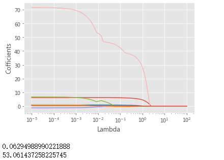
# 绘制Lambda与回归系数的关系
plt.plot(Lambdas, lasso_cofficients)
# 对x轴作对数变换
plt.xscale('log')
# 设置折线图x轴和y轴标签
plt.xlabel('Lambda')
plt.ylabel('Cofficients')
# 显示图形
plt.show()

# LASSO回归模型的交叉验证
lasso_cv = LassoCV(alphas = Lambdas, normalize=True, cv = 10, max_iter=10000)
lasso_cv.fit(X_train, y_train)
# 输出最佳的lambda值
lasso_best_alpha = lasso_cv.alpha_
print(lasso_best_alpha)
# 基于最佳的lambda值建模
lasso = Lasso(alpha = lasso_best_alpha, normalize=True, max_iter=10000)
lasso.fit(X_train, y_train)
# 返回LASSO回归的系数
pd.Series(index = ['Intercept'] + X_train.columns.tolist(),data = [lasso.intercept_] + lasso.coef_.tolist())

# 预测
lasso_predict = lasso.predict(X_test)
# 预测效果验证
RMSE = np.sqrt(mean_squared_error(y_test,lasso_predict))
print(RMSE)

# 导入第三方模块
from statsmodels import api as sms

# 为自变量X添加常数列1，用于拟合截距项
X_train2 = sms.add_constant(X_train)
X_test2 = sms.add_constant(X_test)

# 构建多元线性回归模型
linear = sms.formula.OLS(y_train, X_train2).fit()
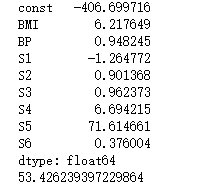
# 返回线性回归模型的系数
print(linear.params)

# 模型的预测
linear_predict = linear.predict(X_test2)
# 预测效果验证
RMSE = np.sqrt(mean_squared_error(y_test,linear_predict))
print(RMSE)