吴裕雄 数据挖掘与分析案例实战（13）——GBDT模型的应用

# 导入第三方包
import pandas as pd
import matplotlib.pyplot as plt

# 读入数据
default = pd.read_excel(r'F:\\python_Data_analysis_and_mining\\14\\default of credit card clients.xls')
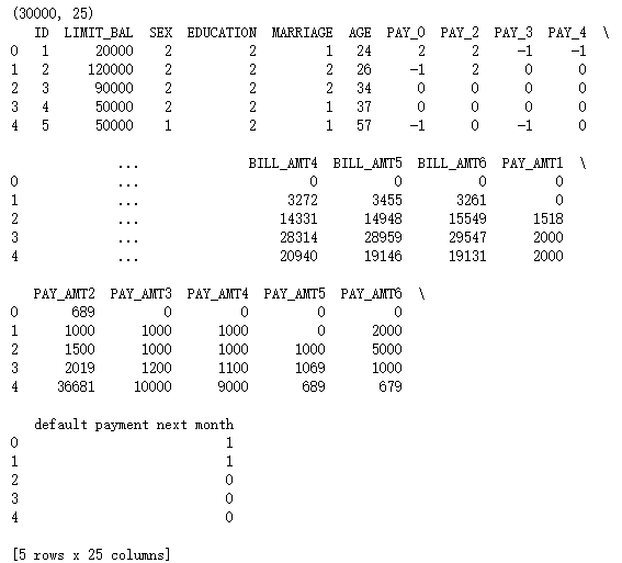
print(default.shape)
print(default.head())
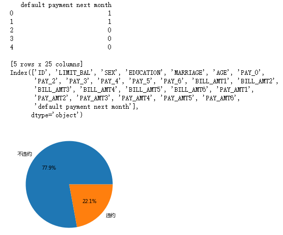
print(default.columns)
# 数据集中是否违约的客户比例
# 为确保绘制的饼图为圆形，需执行如下代码
plt.axes(aspect = 'equal')
# 中文乱码和坐标轴负号的处理
plt.rcParams['font.sans-serif'] = ['Microsoft YaHei']
plt.rcParams['axes.unicode_minus'] = False
# 统计客户是否违约的频数
default['y']=default['default payment next month']
counts = default.y.value_counts()
# 绘制饼图
plt.pie(x = counts, # 绘图数据
labels=pd.Series(counts.index).map({0:'不违约',1:'违约'}), # 添加文字标签
autopct='%.1f%%' # 设置百分比的格式，这里保留一位小数
)
# 显示图形
plt.show()

# 将数据集拆分为训练集和测试集
# 导入第三方包
from sklearn import model_selection
from sklearn import ensemble
from sklearn import metrics

# 排除数据集中的ID变量和因变量，剩余的数据用作自变量X
X = default.drop(['ID','y','default payment next month'], axis = 1)
y = default.y
# 数据拆分
X_train,X_test,y_train,y_test = model_selection.train_test_split(X,y,test_size = 0.25, random_state = 1234)
# 构建AdaBoost算法的类
AdaBoost1 = ensemble.AdaBoostClassifier()
# 算法在训练数据集上的拟合
AdaBoost1.fit(X_train,y_train)
# 算法在测试数据集上的预测
pred1 = AdaBoost1.predict(X_test)

# 返回模型的预测效果
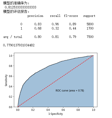
print('模型的准确率为：\n',metrics.accuracy_score(y_test, pred1))
print('模型的评估报告：\n',metrics.classification_report(y_test, pred1))

# 计算客户违约的概率值，用于生成ROC曲线的数据
y_score = AdaBoost1.predict_proba(X_test)[:,1]
fpr,tpr,threshold = metrics.roc_curve(y_test, y_score)
# 计算AUC的值
roc_auc = metrics.auc(fpr,tpr)
print(roc_auc)
# 绘制面积图
plt.stackplot(fpr, tpr, color='steelblue', alpha = 0.5, edgecolor = 'black')
# 添加边际线
plt.plot(fpr, tpr, color='black', lw = 1)
# 添加对角线
plt.plot([0,1],[0,1], color = 'red', linestyle = '--')
# 添加文本信息
plt.text(0.5,0.3,'ROC curve (area = %0.2f)' % roc_auc)
# 添加x轴与y轴标签
plt.xlabel('1-Specificity')
plt.ylabel('Sensitivity')
# 显示图形
plt.show()
# 自变量的重要性排序
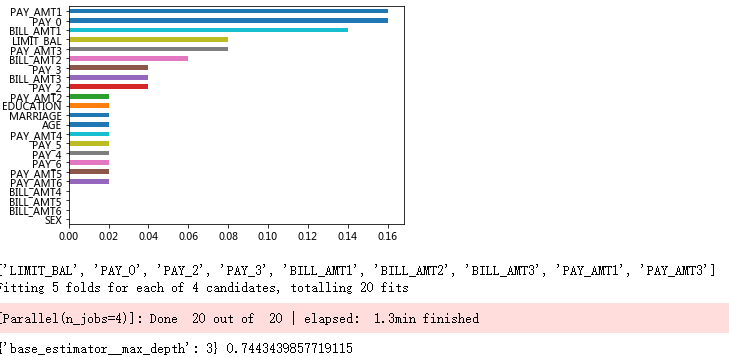
importance = pd.Series(AdaBoost1.feature_importances_, index = X.columns)
importance.sort_values().plot(kind = 'barh')
plt.show()
# 取出重要性比较高的自变量建模
predictors = list(importance[importance>0.02].index)
print(predictors)

# 通过网格搜索法选择基础模型所对应的合理参数组合
# 导入第三方包
from sklearn.model_selection import GridSearchCV
from sklearn.tree import DecisionTreeClassifier

max_depth = [3,4,5,6]
params1 = {'base_estimator__max_depth':max_depth}
base_model = GridSearchCV(estimator = ensemble.AdaBoostClassifier(base_estimator = DecisionTreeClassifier()),
param_grid= params1, scoring = 'roc_auc', cv = 5, n_jobs = 4, verbose = 1)
base_model.fit(X_train[predictors],y_train)
# 返回参数的最佳组合和对应AUC值
print(base_model.best_params_, base_model.best_score_)

# 通过网格搜索法选择提升树的合理参数组合
# 导入第三方包
from sklearn.model_selection import GridSearchCV

n_estimators = [100,200,300]
learning_rate = [0.01,0.05,0.1,0.2]
params2 = {'n_estimators':n_estimators,'learning_rate':learning_rate}
adaboost = GridSearchCV(estimator = ensemble.AdaBoostClassifier(base_estimator = DecisionTreeClassifier(max_depth = 3)),
param_grid= params2, scoring = 'roc_auc', cv = 5, n_jobs = 4, verbose = 1)
adaboost.fit(X_train[predictors] ,y_train)
# 返回参数的最佳组合和对应AUC值
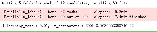
print(adaboost.best_params_, adaboost.best_score_)

# 使用最佳的参数组合构建AdaBoost模型
AdaBoost2 = ensemble.AdaBoostClassifier(base_estimator = DecisionTreeClassifier(max_depth = 3),
n_estimators = 300, learning_rate = 0.01)
# 算法在训练数据集上的拟合
AdaBoost2.fit(X_train[predictors],y_train)
# 算法在测试数据集上的预测
pred2 = AdaBoost2.predict(X_test[predictors])

# 返回模型的预测效果
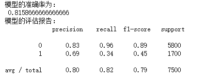
print('模型的准确率为：\n',metrics.accuracy_score(y_test, pred2))
print('模型的评估报告：\n',metrics.classification_report(y_test, pred2))

# 计算正例的预测概率，用于生成ROC曲线的数据
y_score = AdaBoost2.predict_proba(X_test[predictors])[:,1]
fpr,tpr,threshold = metrics.roc_curve(y_test, y_score)
# 计算AUC的值
roc_auc = metrics.auc(fpr,tpr)
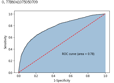
print(roc_auc)
# 绘制面积图
plt.stackplot(fpr, tpr, color='steelblue', alpha = 0.5, edgecolor = 'black')
# 添加边际线
plt.plot(fpr, tpr, color='black', lw = 1)
# 添加对角线
plt.plot([0,1],[0,1], color = 'red', linestyle = '--')
# 添加文本信息
plt.text(0.5,0.3,'ROC curve (area = %0.2f)' % roc_auc)
# 添加x轴与y轴标签
plt.xlabel('1-Specificity')
plt.ylabel('Sensitivity')
# 显示图形
plt.show()

# 运用网格搜索法选择梯度提升树的合理参数组合
learning_rate = [0.01,0.05,0.1,0.2]
n_estimators = [100,300,500]
max_depth = [3,4,5,6]
params = {'learning_rate':learning_rate,'n_estimators':n_estimators,'max_depth':max_depth}
gbdt_grid = GridSearchCV(estimator = ensemble.GradientBoostingClassifier(),
param_grid= params, scoring = 'roc_auc', cv = 5, n_jobs = 4, verbose = 1)
gbdt_grid.fit(X_train[predictors],y_train)
# 返回参数的最佳组合和对应AUC值
print(gbdt_grid.best_params_, gbdt_grid.best_score_)

# 基于最佳参数组合的GBDT模型，对测试数据集进行预测
pred = gbdt_grid.predict(X_test[predictors])
# 返回模型的预测效果
print('模型的准确率为：\n',metrics.accuracy_score(y_test, pred))
print('模型的评估报告：\n',metrics.classification_report(y_test, pred))

# 计算违约客户的概率值，用于生成ROC曲线的数据
y_score = gbdt_grid.predict_proba(X_test[predictors])[:,1]
fpr,tpr,threshold = metrics.roc_curve(y_test, y_score)
# 计算AUC的值
roc_auc = metrics.auc(fpr,tpr)
print(roc_auc)

# 绘制面积图
plt.stackplot(fpr, tpr, color='steelblue', alpha = 0.5, edgecolor = 'black')
# 添加边际线
plt.plot(fpr, tpr, color='black', lw = 1)
# 添加对角线
plt.plot([0,1],[0,1], color = 'red', linestyle = '--')
# 添加文本信息
plt.text(0.5,0.3,'ROC curve (area = %0.2f)' % roc_auc)
# 添加x轴与y轴标签
plt.xlabel('1-Specificity')
plt.ylabel('Sensitivity')
# 显示图形
plt.show()

import numpy as np
import pandas as pd
import matplotlib.pyplot as plt

# 读入数据
creditcard = pd.read_csv(r'F:\\python_Data_analysis_and_mining\\14\\creditcard.csv')
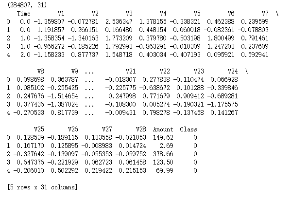
print(creditcard.shape)
print(creditcard.head())
# 为确保绘制的饼图为圆形，需执行如下代码
# 中文乱码和坐标轴负号的处理
plt.rcParams['font.sans-serif'] = ['Microsoft YaHei']
plt.rcParams['axes.unicode_minus'] = False
plt.axes(aspect = 'equal')
# 统计交易是否为欺诈的频数
counts = creditcard.Class.value_counts()
# 绘制饼图
plt.pie(x = counts, # 绘图数据
labels=pd.Series(counts.index).map({0:'正常',1:'欺诈'}), # 添加文字标签
autopct='%.2f%%' # 设置百分比的格式，这里保留一位小数
)
# 显示图形
plt.show()

from sklearn import model_selection

# 将数据拆分为训练集和测试集
# 删除自变量中的Time变量
X = creditcard.drop(['Time','Class'], axis = 1)
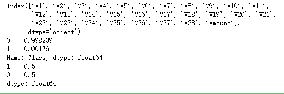
print(X.columns)
y = creditcard.Class
# 数据拆分
X_train,X_test,y_train,y_test = model_selection.train_test_split(X,y,test_size = 0.3, random_state = 1234)

# 导入第三方包
from imblearn.over_sampling import SMOTE

# 运用SMOTE算法实现训练数据集的平衡
over_samples = SMOTE(random_state=1234)
over_samples_X,over_samples_y = over_samples.fit_sample(X_train, y_train)
# over_samples_X,over_samples_y = over_samples.fit_sample(X_train.values,y_train.values.ravel())
# 重抽样前的类别比例
print(y_train.value_counts()/len(y_train))
# 重抽样后的类别比例
print(pd.Series(over_samples_y).value_counts()/len(over_samples_y))

# 导入第三方包
import xgboost
import numpy as np

# 构建XGBoost分类器
xgboost = xgboost.XGBClassifier()
# 使用重抽样后的数据，对其建模
xgboost.fit(over_samples_X,over_samples_y)
# 将模型运用到测试数据集中
resample_pred = xgboost.predict(np.array(X_test))

# 返回模型的预测效果
print('模型的准确率为：\n',metrics.accuracy_score(y_test, resample_pred))
print('模型的评估报告：\n',metrics.classification_report(y_test, resample_pred))

# 计算欺诈交易的概率值，用于生成ROC曲线的数据
y_score = xgboost.predict_proba(np.array(X_test))[:,1]
fpr,tpr,threshold = metrics.roc_curve(y_test, y_score)
# 计算AUC的值
roc_auc = metrics.auc(fpr,tpr)

# 绘制面积图
plt.stackplot(fpr, tpr, color='steelblue', alpha = 0.5, edgecolor = 'black')
# 添加边际线
plt.plot(fpr, tpr, color='black', lw = 1)
# 添加对角线
plt.plot([0,1],[0,1], color = 'red', linestyle = '--')
# 添加文本信息
plt.text(0.5,0.3,'ROC curve (area = %0.2f)' % roc_auc)
# 添加x轴与y轴标签
plt.xlabel('1-Specificity')
plt.ylabel('Sensitivity')
# 显示图形
plt.show()

# 构建XGBoost分类器
xgboost2 = xgboost.XGBClassifier()
# 使用非平衡的训练数据集拟合模型
xgboost2.fit(X_train,y_train)
# 基于拟合的模型对测试数据集进行预测
pred2 = xgboost2.predict(X_test)
# 混淆矩阵
pd.crosstab(pred2,y_test)

# 返回模型的预测效果
print('模型的准确率为：\n',metrics.accuracy_score(y_test, pred2))
print('模型的评估报告：\n',metrics.classification_report(y_test, pred2))

# 计算欺诈交易的概率值，用于生成ROC曲线的数据
y_score = xgboost2.predict_proba(X_test)[:,1]
fpr,tpr,threshold = metrics.roc_curve(y_test, y_score)
# 计算AUC的值
roc_auc = metrics.auc(fpr,tpr)

# 绘制面积图
plt.stackplot(fpr, tpr, color='steelblue', alpha = 0.5, edgecolor = 'black')
# 添加边际线
plt.plot(fpr, tpr, color='black', lw = 1)
# 添加对角线
plt.plot([0,1],[0,1], color = 'red', linestyle = '--')
# 添加文本信息
plt.text(0.5,0.3,'ROC curve (area = %0.2f)' % roc_auc)
# 添加x轴与y轴标签
plt.xlabel('1-Specificity')
plt.ylabel('Sensitivity')
# 显示图形
plt.show()