吴裕雄 数据挖掘与分析案例实战（8）——Logistic回归分类模型

import numpy as np
import pandas as pd
import matplotlib.pyplot as plt

# 自定义绘制ks曲线的函数
def plot_ks(y_test, y_score, positive_flag):
# 对y_test,y_score重新设置索引
y_test.index = np.arange(len(y_test))
#y_score.index = np.arange(len(y_score))
# 构建目标数据集
target_data = pd.DataFrame({'y_test':y_test, 'y_score':y_score})
# 按y_score降序排列
target_data.sort_values(by = 'y_score', ascending = False, inplace = True)
# 自定义分位点
cuts = np.arange(0.1,1,0.1)
# 计算各分位点对应的Score值
index = len(target_data.y_score)*cuts
scores = target_data.y_score.iloc[index.astype('int')]
# 根据不同的Score值，计算Sensitivity和Specificity
Sensitivity = []
Specificity = []
for score in scores:
# 正例覆盖样本数量与实际正例样本量
positive_recall = target_data.loc[(target_data.y_test == positive_flag) & (target_data.y_score>score),:].shape[0]
positive = sum(target_data.y_test == positive_flag)
# 负例覆盖样本数量与实际负例样本量
negative_recall = target_data.loc[(target_data.y_test != positive_flag) & (target_data.y_score<=score),:].shape[0]
negative = sum(target_data.y_test != positive_flag)
Sensitivity.append(positive_recall/positive)
Specificity.append(negative_recall/negative)
# 构建绘图数据
plot_data = pd.DataFrame({'cuts':cuts,'y1':1-np.array(Specificity),'y2':np.array(Sensitivity),
'ks':np.array(Sensitivity)-(1-np.array(Specificity))})
# 寻找Sensitivity和1-Specificity之差的最大值索引
max_ks_index = np.argmax(plot_data.ks)
plt.plot([0]+cuts.tolist()+[1], [0]+plot_data.y1.tolist()+[1], label = '1-Specificity')
plt.plot([0]+cuts.tolist()+[1], [0]+plot_data.y2.tolist()+[1], label = 'Sensitivity')
# 添加参考线
plt.vlines(plot_data.cuts[max_ks_index], ymin = plot_data.y1[max_ks_index],
ymax = plot_data.y2[max_ks_index], linestyles = '--')
# 添加文本信息
plt.text(x = plot_data.cuts[max_ks_index]+0.01,
y = plot_data.y1[max_ks_index]+plot_data.ks[max_ks_index]/2,
s = 'KS= %.2f' %plot_data.ks[max_ks_index])
# 显示图例
plt.legend()
# 显示图形
plt.show()

# 导入虚拟数据
virtual_data = pd.read_excel(r'F:\\python_Data_analysis_and_mining\\09\\virtual_data.xlsx')
print(virtual_data.shape)
# 应用自定义函数绘制k-s曲线
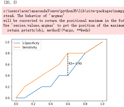
plot_ks(y_test = virtual_data.Class, y_score = virtual_data.Score,positive_flag = 'P')

# 导入第三方模块
import pandas as pd
import numpy as np
from sklearn import linear_model,model_selection

# 读取数据
sports = pd.read_csv(r'F:\\python_Data_analysis_and_mining\\09\\Run or Walk.csv')
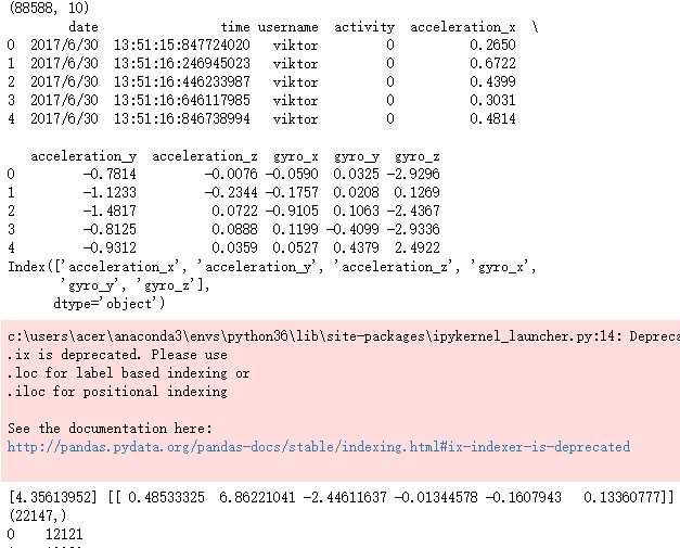
print(sports.shape)
print(sports.head())
# 提取出所有自变量名称
predictors = sports.columns[4:]
print(predictors)
# 构建自变量矩阵
X = sports.ix[:,predictors]
# 提取y变量值
y = sports.activity
# 将数据集拆分为训练集和测试集
X_train, X_test, y_train, y_test = model_selection.train_test_split(X, y, test_size = 0.25, random_state = 1234)
# 利用训练集建模
sklearn_logistic = linear_model.LogisticRegression()
sklearn_logistic.fit(X_train, y_train)
# 返回模型的各个参数
print(sklearn_logistic.intercept_, sklearn_logistic.coef_)
# 模型预测
sklearn_predict = sklearn_logistic.predict(X_test)
print(sklearn_predict.shape)
# 预测结果统计
a = pd.Series(sklearn_predict).value_counts()
print(a)
# 导入第三方模块
from sklearn import metrics

# 混淆矩阵
cm = metrics.confusion_matrix(y_test, sklearn_predict, labels = [0,1])
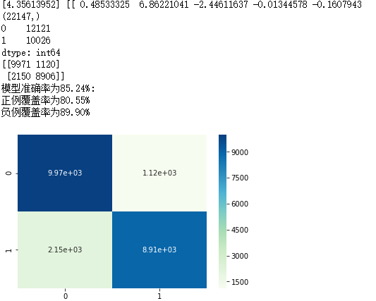
print(cm)
Accuracy = metrics.scorer.accuracy_score(y_test, sklearn_predict)
Sensitivity = metrics.scorer.recall_score(y_test, sklearn_predict)
Specificity = metrics.scorer.recall_score(y_test, sklearn_predict, pos_label=0)
print('模型准确率为%.2f%%:' %(Accuracy*100))
print('正例覆盖率为%.2f%%' %(Sensitivity*100))
print('负例覆盖率为%.2f%%' %(Specificity*100))
# 混淆矩阵的可视化
# 导入第三方模块
import seaborn as sns
import matplotlib.pyplot as plt

# 绘制热力图
sns.heatmap(cm, annot = True, fmt = '.2e',cmap = 'GnBu')
# 图形显示
plt.show()

# y得分为模型预测正例的概率
y_score = sklearn_logistic.predict_proba(X_test)[:,1]
# 计算不同阈值下，fpr和tpr的组合值，其中fpr表示1-Specificity，tpr表示Sensitivity
fpr,tpr,threshold = metrics.roc_curve(y_test, y_score)
# 计算AUC的值
roc_auc = metrics.auc(fpr,tpr)
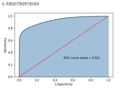
print(roc_auc)
# 绘制面积图
plt.stackplot(fpr, tpr, color='steelblue', alpha = 0.5, edgecolor = 'black')
# 添加边际线
plt.plot(fpr, tpr, color='black', lw = 1)
# 添加对角线
plt.plot([0,1],[0,1], color = 'red', linestyle = '--')
# 添加文本信息
plt.text(0.5,0.3,'ROC curve (area = %0.2f)' % roc_auc)
# 添加x轴与y轴标签
plt.xlabel('1-Specificity')
plt.ylabel('Sensitivity')
# 显示图形
plt.show()

# 调用自定义函数，绘制K-S曲线
plot_ks(y_test = y_test, y_score = y_score, positive_flag = 1)

# -----------------------第一步 建模 ----------------------- #
# 导入第三方模块
import statsmodels.api as sm

# 将数据集拆分为训练集和测试集
X_train, X_test, y_train, y_test = model_selection.train_test_split(X, y, test_size = 0.25, random_state = 1234)
# 为训练集和测试集的X矩阵添加常数列1
X_train2 = sm.add_constant(X_train)
X_test2 = sm.add_constant(X_test)
# 拟合Logistic模型
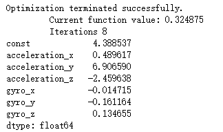
sm_logistic = sm.formula.Logit(y_train, X_train2).fit()
# 返回模型的参数
print(sm_logistic.params)

# -----------------------第二步 预测构建混淆矩阵 ----------------------- #
# 模型在测试集上的预测
sm_y_probability = sm_logistic.predict(X_test2)
# 根据概率值，将观测进行分类，以0.5作为阈值
sm_pred_y = np.where(sm_y_probability >= 0.5, 1, 0)
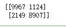
# 混淆矩阵
cm = metrics.confusion_matrix(y_test, sm_pred_y, labels = [0,1])
print(cm)

# -----------------------第三步 绘制ROC曲线 ----------------------- #
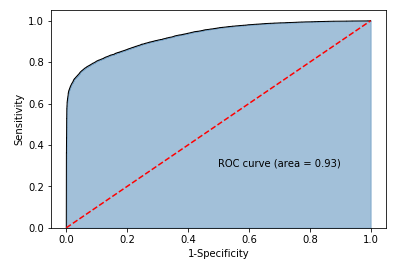
# 计算真正率和假正率
fpr,tpr,threshold = metrics.roc_curve(y_test, sm_y_probability)
# 计算auc的值
roc_auc = metrics.auc(fpr,tpr)
# 绘制面积图
plt.stackplot(fpr, tpr, color='steelblue', alpha = 0.5, edgecolor = 'black')
# 添加边际线
plt.plot(fpr, tpr, color='black', lw = 1)
# 添加对角线
plt.plot([0,1],[0,1], color = 'red', linestyle = '--')
# 添加文本信息
plt.text(0.5,0.3,'ROC curve (area = %0.2f)' % roc_auc)
# 添加x轴与y轴标签
plt.xlabel('1-Specificity')
plt.ylabel('Sensitivity')
# 显示图形
plt.show()

# -----------------------第四步 绘制K-S曲线 ----------------------- #
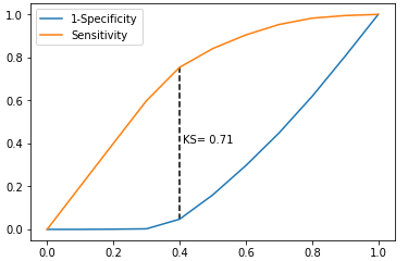
# 调用自定义函数，绘制K-S曲线
sm_y_probability.index = np.arange(len(sm_y_probability))
plot_ks(y_test = y_test, y_score = sm_y_probability, positive_flag = 1)